Chapter 15 LA1: Systems of Linear Equations

Section 15.1 Introduction

An equation such as
\begin{equation*} a_1x_1+a_2x_2+\dots+a_nx_n=b \end{equation*}
(where the \(a_i\) and \(b\) are numbers and the \(x_i\) are variables) is a linear equation in \(n\) variables, (or \(n\) unknowns). In the special case in which \(b=0\) the equation is called homogeneous. (Of course when there are only a small number of variables, \(2\) or \(3\) say, it is common to use completely different labels (such as \(x\text{,}\) \(y\) and \(z\)) for the variables rather than to use subscripts (such as \(x_1\text{,}\) \(x_2\) and \(x_3\)).)

Definition 15.1.

A system of linear equations is a set of \(m\) simultaneous linear equations in \(n\) variables, i.e.
\begin{align*} a_{11}x_1+a_{12}x_2+\dots+a_{1n}x_n \amp =b_1\\ a_{21}x_1+a_{22}x_2+\dots+a_{2n}x_n \amp =b_2\\ \vdots\\ a_{m1}x_1+a_{m2}x_2+\dots+a_{mn}x_n \amp =b_m \end{align*}
A solution to a system of linear equations is a set of values for the variables \(x_1, x_2, \dots, x_n\) that satisfy all of the equations in the system. The solution set to the system is the set of all possible solutions.

Example 15.2.

The following is a homogeneous system of three linear equations in four unknowns.
\begin{align*} 3x_1-x_2+2x_3+x_4 \amp =0\\ -x_1+6x_2-11x_4 \amp =0\\ x_1+x_2+7x_3+4x_4 \amp =0 \end{align*}
A solution to this system of equations is \(x_1=1\text{,}\) \(x_2=2\text{,}\) \(x_3=-1\text{,}\) \(x_4=1\) which can be written as
\begin{equation*} (x_1,x_2,x_3,x_4)=(1,2,-1,1) \end{equation*}
The solution set for this system is the set of points
\begin{equation*} (x_1,x_2,x_3,x_4)=(t,2t,-t,t) \textrm{ where } t\in \mathbb{R} \end{equation*}
You should already be familiar with solving systems of linear equations involving two equations in two variables and interpreting the solution in terms of lines in the plane.

Example 15.3.

Solve the following system of linear equations and interpret the answer geometrically
\begin{align*} 2x-3y \amp =13\\ x-y \amp =5 \end{align*}
Answer.
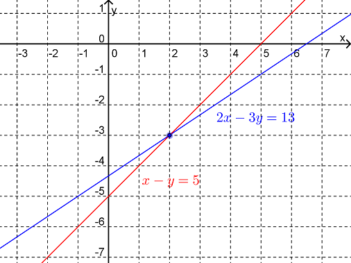
We can interpret the solution \((x,y)=(2,-3)\) as the point in the plane at which the straight lines represented by the equations \(2x-3y=13\) and \(x-y=5\) intersect.
Solution.
Multiplying the second equation by \(2\) and then subtracting this from the first equation gives \(y=-3\text{.}\) Substituting this result into either of the original equations gives \(x=2\text{.}\) Thus the solution is \((x,y)=(2,-3)\text{.}\)
As shown in Figure 15.4, we can interpret the solution \((x,y)=(2,-3)\) as the point in the plane at which the straight lines represented by the equations \(2x-3y=13\) and \(x-y=5\) intersect.
Figure 15.4. Plots of \(2x-3y=13\) (blue) and \(x-y=5\) (red).

Example 15.5.

Solve the following system of linear equations and interpret the answer geometrically
\begin{align*} 2x+3y \amp =4\\ 4x+6y \amp =8 \end{align*}
Answer.
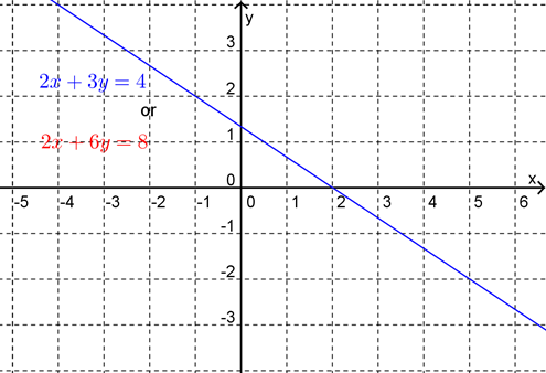
The solution set is \((x,y)=\left(t,\frac{4}{3}-\frac{2}{3}t\right)\text{.}\) The geometric interpretation of this system of linear equations is that both equations represent the same line.
Solution.
Multiplying the first equation by \(2\) and then subtracting this from the second equation gives \(0=0\text{.}\) This tells us that any values of \(x\) and \(y\) that satisfy the first equation will also satisfy the second equation. Thus there are infinitely many solutions. We may choose \(x\) (say) to be anything we like, and then find a corresponding value for \(y\) (from either equation). So if we set \(x=t\text{,}\) then
\begin{equation*} y=\frac{4}{3}-\frac{2}{3}t \end{equation*}
and the solution set is
\begin{equation*} (x,y)=\left(t,\frac{4}{3}-\frac{2}{3}t\right) \end{equation*}
Thus, the parameter \(t\) labels the infinite family of solutions.
The geometric interpretation of this system of linear equations is that both equations represent the same line (as shown in Figure 15.6).
Figure 15.6. Plots of \(2x+3y=4\) (blue) and \(4x+6y=8\) (red).
Note that the solution written in terms of the parameter \(t\) can be interpreted as a vector equation for the line. By writing the solution as
\begin{equation*} (x,y)=\left(0,\frac{4}{3}\right)+t\left(1,-\frac{2}{3}\right) \end{equation*}
we can see that the line passes through the point \(\left(0,\frac{4}{3}\right)\) and is parallel to the vector \(\left(1,-\frac{2}{3}\right)\text{.}\)

Example 15.7.

Solve the following system of linear equations and interpret the answer geometrically
\begin{align*} 2x-3y \amp =13\\ 4x-6y \amp =5 \end{align*}
Answer.
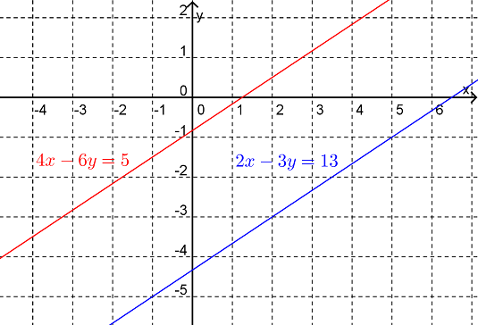
There are no solutions. Geometrically, this system of linear equations can be interpreted as two parallel lines in the plane.
Solution.
Multiplying the first equation by \(2\) and then subtracting this from the second equation gives \(0=-21\text{.}\) This tells us that no values of \(x\) and \(y\) will satisfy these equations. Thus there are no solutions. A system of equations with no solution is said to be inconsistent.
Geometrically, this system of linear equations can be interpreted as two parallel lines in the plane, as shown in Figure 15.8.
Figure 15.8. Plots of \(2x-3y=13\) (blue) and \(4x-6y=5\) (red).
The above (simple) examples illustrate two important facts that hold for all systems of linear equations. Firstly:

Definition 15.9.

A system of \(m\) linear equations in \(n\) unknowns has either
  • A unique solution,
  • An infinite number of solutions, or
  • No solution
Thus it is impossible, for example, for a system of linear equations to have exactly two or exactly three solutions. (We will see why this is later.) Secondly, we cannot tell which of these cases (i.e. a unique solution, infinitely many solutions or no solution) applies simply by counting the number of equations and unknowns.
For systems of two linear equations in two unknowns we have seen that we can solve the system via the "substitution method" (viz. making one variable the subject of one equation and then substituting this into the second equation) or the "elimination method" (viz. adding a multiple of one equation to other). For larger system of equations this basic idea can still be used but the working can be become quite messy. In the following sections we will look at a systematic way of solving a system of \(m\) linear equations in \(n\) unknowns using matrices.

Section 15.2 Matrices and Systems of Linear Equations

Definition 15.10.

An \(m\times n\) matrix is a rectangular array of numbers with \(m\) rows and \(n\) columns, i.e.
\begin{equation*} \begin{pmatrix} a_{11} \amp a_{12} \amp \dots \amp a_{1n} \\ a_{21} \amp a_{22} \amp \dots \amp a_{2n} \\ \vdots \amp \vdots \amp \ddots \amp \vdots \\ a_{m1} \amp a_{m2} \amp \dots \amp a_{mn} \end{pmatrix}=(a_{ij})_{m\times n} \end{equation*}
We say that the number \(a_{ij}\) is the \((i,j)\)th entry (i.e. the entry in row \(i\text{,}\) column \(j\)).

Example 15.11.

The following are examples of matrices.
\begin{equation*} \begin{pmatrix} 1 \amp 2 \amp 3 \\ 4 \amp 5 \amp 10 \end{pmatrix} \hspace{5mm} \begin{pmatrix} 0 \amp \frac{1}{4} \\ -\frac{1}{2} \amp 3 \end{pmatrix} \hspace{5mm} \begin{pmatrix} \sqrt{2} \\ 1 \\ -3 \end{pmatrix} \end{equation*}
\begin{equation*} \hspace{5mm} 2\times 3 \textrm{ matrix } \hspace{5mm} 2\times 2 \textrm{ matrix } \hspace{4mm} 3\times 1 \textrm{ matrix } \end{equation*}
Matrices have proved useful in many areas of mathematics and we will study them in more detail throughout this strand. With respect to the following system of linear equations
\begin{align*} a_{11}x_1+a_{12}x_2+\dots+a_{1n}x_n \amp =b_1\\ a_{21}x_1+a_{22}x_2+\dots+a_{2n}x_n \amp =b_2\\ \vdots \\ a_{m1}x_1+a_{m2}x_2+\dots+a_{mn}x_n \amp =b_m \end{align*}
so long as the variables are always written in the same order and the constants are always put on to the right hand side we can represent this system via the \(m\times (n+1)\) matrix
\begin{equation*} \begin{pmatrix} a_{11} \amp a_{12} \amp \dots \amp a_{1n} \amp b_{1} \\ a_{21} \amp a_{22} \amp \dots \amp a_{2n} \amp b_{2} \\ \vdots \amp \vdots \amp \ddots \amp \vdots \amp \vdots \\ a_{m1} \amp a_{m2} \amp \dots \amp a_{mn} \amp b_m \end{pmatrix} \end{equation*}
This matrix is called the augmented matrix for the system of linear equations. Each row of this matrix corresponds to an equation in the system. Each of the first \(n\) columns corresponds to the coefficients of a variable in the equations and the last column gives the constants on the right hand sides of the equations.

Example 15.12.

Write down the augmented matrix for the following non-homogenous system of linear equations
\begin{align*} 3x_1-x_2+2x_3+x_4 \amp =2\\ -x_1+6x_2-11x_4 \amp =-22\\ x_1+x_2+7x_3+4x_4 \amp =8 \end{align*}
Solution.
The augmented matrix will be the \(3\times 5\) matrix
\begin{equation*} \begin{pmatrix} 3 \amp -1 \amp 2 \amp 1 \amp 2 \\ -1 \amp 6 \amp 0 \amp -11 \amp -22 \\ 1 \amp 1 \amp 7 \amp 4 \amp 8 \end{pmatrix} \end{equation*}
Note that sometimes a partition line is put before the last column in an augmented matrix to emphasise that the last column represents the right hand side of the equations while the remaining columns represent the coefficients of the variables in the system. The matrix without the last column is called the coefficient matrix for the system of equations.

Example 15.13. (Example 15.12 cont.).

For this system of linear equations the augmented matrix is sometimes written as
\begin{equation*} \left(\begin{array}{c c c c | c} 3 \amp -1 \amp 2 \amp 1 \amp 2 \\ -1 \amp 6 \amp 0 \amp -11\amp -22 \\ 1 \amp 1 \amp 7 \amp 4 \amp 8 \end{array}\right) \end{equation*}
The coefficient matrix for this system is
\begin{equation*} \begin{pmatrix} 3 \amp -1 \amp 2 \amp 1 \\ -1 \amp 6 \amp 0 \amp -11 \\ 1 \amp 1 \amp 7 \amp 4 \end{pmatrix} \end{equation*}

Example 15.14.

Write down the system of linear equations that correspond to the following augmented matrices.
  1. \begin{equation*} \left(\begin{array}{c c c | c} 3 \amp -2 \amp 2 \amp -3 \\ -1 \amp 6 \amp 4 \amp 7 \\ 1 \amp 1 \amp 5 \amp -2 \end{array}\right) \end{equation*}
  2. \begin{equation*} \left(\begin{array}{c c c | c} 1 \amp 0 \amp 0 \amp 1 \\ 0 \amp 1 \amp 0 \amp 2 \\ 0 \amp 0 \amp 1 \amp -1 \end{array}\right) \end{equation*}
Solution.
  1. Calling the variables as \(x\text{,}\) \(y\) and \(z\) the system of equations is
    \begin{align*} 3x-2y+2z \amp =-3\\ -x+6y+4z \amp =7\\ x+y+5z \amp =-2 \end{align*}
  2. Again calling the variables \(x\text{,}\) \(y\) and \(z\) this augmented matrix represents the very simple system of equations
    \begin{align*} x \amp =1\\ y \amp =2\\ z \amp =-1 \end{align*}

Section 15.3 Solving Systems of Linear Equations

Two systems of linear equations are said to be equivalent if they have the same number of variables and have the same solution sets.

Example 15.15. (Example 15.14 cont.).

It turns out that the systems of linear equations in Example 15.14 are equivalent, i.e.
\begin{align*} 3x-2y+2z \amp =-3 \hspace{48mm} x=1\\ -x+6y+4z \amp =7 \hspace{10mm} \textrm{ is equivalent to } \hspace{10mm} y=2\\ x+y+5z \amp =-2 \hspace{49mm} z=-1 \end{align*}
The solution to these equivalent systems can be seen from the system on the right whereas they are not at all obvious from the system on the left.
Notice that, given a system of linear equations, we can produce an equivalent system by doing any one of the following:
  • Multiplying any one equation by a non-zero constant
  • Re-writing the equations in a different order
  • Adding any multiple of one equation to another

Example 15.16.

The following systems of linear equations are equivalent because we have just written the equations in a different order.
\begin{align*} 3x-2y+2z \amp =-3 \hspace{52mm} 3x-2y+2z =-3\\ -x+6y+4z \amp =7 \hspace{10mm} \textrm{ is equivalent to } \hspace{18mm} x+y+5z =-2\\ x+y+5z \amp =-2 \hspace{48mm} -x+6y+4z =7 \end{align*}
The following systems of linear equations are equivalent because we have just multiplied the second equation by \(3\text{.}\)
\begin{align*} 3x-2y+2z \amp =-3 \hspace{54mm} 3x-2y+2z =-3\\ x+y+5z \amp =-2 \hspace{10mm} \textrm{ is equivalent to } \hspace{9mm} 3x+3y+15z =-6\\ -x+6y+4z \amp =7 \hspace{54mm} -x+6y+4z =7 \end{align*}
The following systems of linear equations are equivalent because we have just subtracted the first equation from the second equation, (i.e. added \(-1\) times the first equation to the second equation.)
\begin{align*} 3x-2y+2z \amp =-3 \hspace{48mm} 3x-2y+2z =-3\\ 3x+3y+15z \amp =-6 \hspace{10mm} \textrm{ is equivalent to } \hspace{15mm} 5y+13z =-3\\ -x+6y+4z \amp =7 \hspace{49mm} -x+6y+4z =7 \end{align*}
Thus the strategy for solving a system of linear equations will be to apply the above operations in a systematic way to produce an equivalent system from which we can determine the solution (such as that given in Example 15.14\((b)\)). This strategy, in the form described below, is called Gauss-Jordon Elimination. In order to describe this strategy we need some terminology.

Definition 15.17.

Given a matrix an equivalent matrix can be produced by applying any one of the following three elementary row operations:
  • Swapping two rows
  • Multiplying a row by a non-zero constant
  • Adding a multiple of one row to another row
Note:
  1. We use the symbol \(\sim\) to denote that two matrices are equivalent.
  2. The process of applying elementary row operations to a matrix is called row reduction

Example 15.18. (Example 15.16 cont.).

The following matrices are equivalent because we have just swapped two rows.
\begin{equation*} \left(\begin{array}{c c c | c} 3 \amp -2 \amp 2 \amp -3 \\ -1 \amp 6 \amp 4 \amp 7 \\ 1 \amp 1 \amp 5 \amp -2 \end{array}\right) \sim \left(\begin{array}{c c c | c} 3 \amp -2 \amp 2 \amp -3 \\ 1 \amp 1 \amp 5 \amp -2 \\ -1 \amp 6 \amp 4 \amp 7 \end{array}\right) \begin{matrix} \\ \hspace{5mm} R_2'=R_3 \\ \hspace{5mm} R_3'=R_2 \end{matrix} \end{equation*}
The following matrices are equivalent because we have just multiplied Row \(2\) by \(3\text{.}\)
\begin{equation*} \left(\begin{array}{c c c | c} 3 \amp -2 \amp 2 \amp -3 \\ 1 \amp 1 \amp 5 \amp -2 \\ -1 \amp 6 \amp 4 \amp 7 \end{array}\right) \sim \left(\begin{array}{c c c | c} 3 \amp -2 \amp 2 \amp -3 \\ 3 \amp 3 \amp 15 \amp -6 \\ -1 \amp 6 \amp 4 \amp 7 \end{array}\right) \hspace{5mm} R_2'=3R_2 \end{equation*}
The following matrices are equivalent because we have just subtracted Row \(1\) from Row \(2\text{,}\) (i.e. added \(-1\) times Row \(1\) to Row \(2\))
\begin{equation*} \left(\begin{array}{c c c | c} 3 \amp -2 \amp 2 \amp -3 \\ 3 \amp 3 \amp 15 \amp -6 \\ -1 \amp 6 \amp 4 \amp 7 \end{array}\right) \sim \left(\begin{array}{c c c | c} 3 \amp -2 \amp 2 \amp -3 \\ 0 \amp 5 \amp 13 \amp -3 \\ -1 \amp 6 \amp 4 \amp 7 \end{array}\right) \hspace{5mm} R_2'=R_2-R_1 \end{equation*}

Definition 15.19.

A matrix is said to be in row-echelon form if the first non-zero entry (i.e. the leading entry) in each row occurs further to the right than in the row above it.
A matrix is said to be in reduced row-echelon form if it is in row-echelon form and each leading entry is 1 with no non-zero entries above it.

Example 15.20.

For the following matrices decide if it is row-echelon form, reduced row-echelon form or neither. For those matrices in reduced row-echelon form what can you say about the system of linear equations represented by those matrices?
  1. \begin{equation*} \begin{pmatrix} 1 \amp 0 \amp 3 \amp 2 \\ 0 \amp 1 \amp -1 \amp -3 \\ 0 \amp 0 \amp 0 \amp 0 \end{pmatrix} \end{equation*}
  2. \begin{equation*} \left(\begin{array}{c c c c | c} 3 \amp -1 \amp 2 \amp 1 \amp 2 \\ 0 \amp 7 \amp 7 \amp -7 \amp -16 \\ 1 \amp 1 \amp 7 \amp 4 \amp 8 \end{array}\right) \end{equation*}
  3. \begin{equation*} \begin{pmatrix} 1 \amp 4 \amp -1 \amp 2 \\ 0 \amp 2 \amp 3 \amp -2 \\ 0 \amp 0 \amp 4 \amp 5 \\ 0 \amp 0 \amp 0 \amp 6 \end{pmatrix} \end{equation*}
  4. \begin{equation*} \begin{pmatrix} 1 \amp 0 \amp 0 \amp 1 \\ 0 \amp 1 \amp 0 \amp 2 \\ 0 \amp 0 \amp 1 \amp -1 \end{pmatrix} \end{equation*}
Solution.
  1. This matrix is in reduced row-echelon form. The system of equations represented by this matrix is
    \begin{align*} x+3z \amp =2\\ y-z \amp =-3\\ 0 \amp =0 \end{align*}
    The third equation in this system is satisfied no matter what values we choose for \(x\text{,}\) \(y\) and \(z\text{.}\) Once we choose a value for \(z\) (say) then from the first two equations we can determine the values for \(x\) and \(y\) as
    \begin{align*} x \amp =2-3z\\ y \amp =-3+z \end{align*}
    Thus this system of equations has an infinite number of solutions given by
    \begin{equation*} (x,y,z)=(2-3t,-3+t,t) \end{equation*}
    or
    \begin{equation*} (x,y,z)=(2,-3,0)+t(-3,1,1) \end{equation*}
  2. This matrix isn’t in row-echelon form (and hence not in reduced row-echelon form either) since the leading entry in row \(3\) occurs to the left of the leading entry is row \(2\text{.}\)
  3. This matrix is in row-echelon form but not reduced row-echelon form. Notice that in this case we can tell that the associated system of linear equations is inconsistent even though the matrix is not in reduced row-echelon form. The fourth equation in this system is
    \begin{equation*} 0=6 \end{equation*}
    and this cannot be satisfied no matter which values of \(x\text{,}\) \(y\) and \(z\) we choose.
  4. This matrix is in reduced row-echelon form and the solution of the associated systems of linear equations is
    \begin{equation*} (x,y,z)=(1,2,-1) \end{equation*}

Definition 15.21.

In Gauss-Jordon Elimination, the augmented matrix associated with the system of linear equations is systematically row reduced to reduced row-echelon form by:
  • Obtaining a 1 in entry \(a_{11}\)
  • Obtaining \(0\)’s in the remainder of column \(1\) by using the elementary row operation of adding multiples of row \(1\) to another row.
  • Obtaining a 1 in entry \(a_{22}\)
  • Obtaining \(0\)’s in the remainder of column \(2\) by using the elementary row operation of adding multiples of row \(2\) to another row.
  • And so on across the columns.
The solution is then read off from the equivalent system represented by the matrix in reduced row-echelon form

Example 15.22.

Use Gauss Jordon Elimination to solve the following system of linear equations:
\begin{align*} 2x+3y \amp =1\\ 3x-4y \amp =10 \end{align*}
Solution.
The augmented matrix for this system is
\begin{equation*} \left(\begin{array}{c c | c} 2 \amp 3 \amp 1 \\ 3 \amp -4 \amp 10 \end{array}\right) \end{equation*}
We now want to row reduce this matrix to reduced row-echelon form. Following the steps as outlined:
\begin{align*} \begin{pmatrix} 2 \amp 3 \amp 1 \\ 3 \amp -4 \amp 10 \end{pmatrix} \amp \sim \begin{pmatrix} 1 \amp \frac{3}{2} \amp \frac{1}{2} \\ 0 \amp -\frac{17}{2} \amp \frac{17}{2} \end{pmatrix} \begin{matrix} R_1'=R_1/2 \\ \hspace{8mm} R_2'=R_2-3R_1' \end{matrix}\\ \amp \sim \begin{pmatrix} 1 \amp 0 \amp 2 \\ 0 \amp 1 \amp -1 \end{pmatrix} \begin{matrix} \hspace{15mm} R_1'=R_1-3R_2'/2 \\ \hspace{10mm} R_2'=-2R_2/17 \end{matrix} \end{align*}
We can now read off the solution as
\begin{equation*} (x,y)=(2,-1) \end{equation*}
Of course we can check that this solution is correct by substituting these values into the original equations.
In doing the row reduction here were had to use fractions. It is possible to apply the elementary row operations in a manner that avoids the fractions until the last steps. However you have to be very careful in doing this that you don’t lose some of the \(0\)’s that you have already created and hence start going around in circles!
Example 15.23.

Use Gauss Jordon Elimination to solve the following system of linear equations.
\begin{align*} 2x+6y+2z \amp = 4\\ 3x+2y+z \amp = 0\\ 2x+3y \amp = 1 \end{align*}
Solution.
The augmented matrix for this system is
\begin{equation*} \begin{pmatrix} 2 \amp 6 \amp 2 \amp 4 \\ 3 \amp 2 \amp 1 \amp 0 \\ 2 \amp 3 \amp 0 \amp 1 \end{pmatrix} \end{equation*}
Now using the steps as outlined to reduce this to reduced row-echelon form:
\begin{align*} \begin{pmatrix} 2 \amp 6 \amp 2 \amp 4 \\ 3 \amp 2 \amp 1 \amp 0 \\ 2 \amp 3 \amp 0 \amp 1 \end{pmatrix} \amp \sim \begin{pmatrix} 1 \amp 3 \amp 1 \amp 2 \\ 0 \amp -7 \amp -2 \amp -6 \\ 0 \amp -3 \amp -2 \amp -3 \end{pmatrix} \begin{matrix} R_1'=R_1/2 \\ \hspace{10mm} R_2'=R_2-3R_1' \\ \hspace{10mm} R_3'=R_3-2R_1' \end{matrix} \\ \amp \sim \begin{pmatrix} 1 \amp 0 \amp \frac{1}{7} \amp -\frac{4}{7} \\ 0 \amp 1 \amp \frac{2}{7} \amp \frac{6}{7} \\ 0 \amp 0 \amp -\frac{8}{7} \amp -\frac{3}{7} \end{pmatrix} \hspace{6mm} \begin{matrix} \hspace{5mm} R_1'=R_1-3R_2' \\ R_2'=-R_2/7 \\ \hspace{5.5mm} R_3'=R_3+3R_2' \end{matrix}\\ \amp \sim \begin{pmatrix} 1 \amp 0 \amp 0 \amp -\frac{5}{8} \\ 0 \amp 1 \amp 0 \amp \frac{3}{4} \\ 0 \amp 0 \amp 1 \amp \frac{3}{8} \end{pmatrix} \begin{matrix} \hspace{14.5mm} R_1'=R_1-R_3'/7 \\ \hspace{16.5mm} R_2'=R_2-2R_3'/7 \\ \hspace{10mm} R_3'=-7R_3/8 \end{matrix} \end{align*}
Thus the solution is
\begin{equation*} (x,y,z)=\left(-\frac{5}{8},\frac{3}{4},\frac{3}{8}\right) \end{equation*}

Exercises Example Tasks

1.
For the following augmented matrices write down the general solution of the associated system of linear equations, (i.e. write down the set of all solutions).
  1. \begin{equation*} \begin{pmatrix} 0 \amp 2 \amp 2 \amp 2 \\ 0 \amp 0 \amp 3 \amp 3\end{pmatrix} \end{equation*}
  2. \begin{equation*} \begin{pmatrix} 1 \amp 0 \amp 0 \amp 2 \\ 0 \amp 1 \amp 0 \amp 3 \\ 0 \amp 0 \amp 0 \amp 0 \end{pmatrix} \end{equation*}
  3. \begin{equation*} \begin{pmatrix} 1 \amp -1 \amp 2 \amp 3 \\ 0 \amp 0 \amp 0 \amp 0 \\ 0 \amp 0 \amp 0 \amp 0 \end{pmatrix} \end{equation*}
  4. \begin{equation*} \begin{pmatrix} 1 \amp -6 \amp 0 \amp 0 \amp 3 \amp -2 \\ 0 \amp 0 \amp 1 \amp 0 \amp 4 \amp 7 \\ 0 \amp 0 \amp 0 \amp 1 \amp 5 \amp 8 \\ 0 \amp 0 \amp 0 \amp 0 \amp 0 \amp 0 \end{pmatrix} \end{equation*}
2.
Solve the following system of linear equations by Gauss-Jordan elimination.
\begin{align*} 5x+2y-z \amp =11\\ x-y+z \amp =1\\ 4x+2y+3z \amp =5 \end{align*}
3.
The general equation of a circle is \(x^2+y^2+ax+by+c=0\text{.}\) Find the equation of the circle that passes through the points \((1,0)\text{,}\) \((2,1)\) and \((2,-1)\text{.}\)