DE2: First Order Separable DEs

Chapter 10 DE2: First Order Separable DEs

In Chapter 9 we discussed the concept of a differential equation and saw how to check if a function is a solution of a given DE. However, except for the case where the DE is of the form

\begin{equation*} y^{(n)}(x)=f(x) \end{equation*}

(where we can find the solutions just by integration) we have not yet seen any algebraic methods for finding the solutions to a DE. (We did see that for first order DEs we can obtain a graphical representation of the solutions via a direction field and a numerical approximation to a particular solution via Euler’s method.)

As mentioned in Chapter 9 there is no one general method that will solve all possible DEs. However, for various classes of DEs methods have been found that will find their solution. In this lecture we are going to look at an algebraic method for finding the solutions to the class of DEs called first order separable DEs.

Section 10.1 First Order Separable DEs

Definition 10.1.

A differential equation of the form

\begin{equation*} \frac{dy}{dx}=f(x)g(y) \end{equation*}

where \(g(y)\neq 0\) is called a first order separable DE.

Example 10.2.

Which of the following DEs are first order separable DEs?

\(\displaystyle y^2y'=x \)
\(\displaystyle y''+2y=0 \)
\(\displaystyle \frac{dy}{dt}+3e^t=ye^t \)
\(\displaystyle \frac{dy}{dt}+ty=2 \)
\(\displaystyle y'=y(1-y) \)
\(\displaystyle y'=y(x-y) \)

Answer.

\(a\text{,}\) \(c\) and \(e\)

Solution.

This DE can be written as
\begin{equation*} y'=\frac{x}{y^2} \end{equation*}
Thus it is a first order separable DE with \(f(x)=x\) and \(g(y)=\frac{1}{y^2}\text{.}\)
This DE is a second order DE (due to the \(y''\) term) and hence cannot be a first order separable DE.
This DE can be rearranged as
\begin{equation*} \frac{dy}{dt}=e^t(y-3) \end{equation*}
and hence is a first order separable DE with \(f(t)=e^t\) and \(g(y)=y-3\text{.}\)
When we try to rearrange this DE in the same manner as we did in part (c) we obtain
\begin{equation*} \frac{dy}{dt}=2-ty \end{equation*}
This is not of the form \(y'=f(t)g(y)\) and hence this first order DE is not separable.
This DE is already in the form of a first order separable DE with \(f(x)=1\) and \(g(y)=y(1-y)\text{.}\)
The right hand side of this DE can’t be rearranged into the form \(y'=f(x)g(y)\) and so this DE is not a first order separable DE.

The method for solving first order separable DEs is based on integration by substitution. This integration technique was covered in Math1110 but the following example is given as a reminder.

Example 10.3.

Evaluate the integral \(\displaystyle\int 2x\sin(x^2) \hspace{2mm} dx\text{.}\)

Answer.

\(\displaystyle\int 2x\sin(x^2)\hspace{2mm} dx=-\cos(x^2)+C\)

Solution.

Since the integrand is of the form \(g'(x)\sin(g(x))\) (or, in Leibniz notation \(\sin(g(x))\frac{dg}{dx}\)) make the substitution

\begin{equation*} u=g(x)=x^2 \end{equation*}

Then

\begin{align*} \int 2x\sin(x^2)\hspace{2mm} dx \amp =\int \sin(u)\hspace{2mm} du\\ \amp =-\cos(u)+C \end{align*}

Using \(u=x^2\) gives

\begin{equation*} \int 2x\sin(x^2)\hspace{2mm} dx=-\cos(x^2)+C \end{equation*}

In general, the integration by substitution method says that for an integral of the form

\begin{equation*} \int f(g(x))\frac{dg}{dx}\hspace{2mm} dx \end{equation*}

the substitution

\begin{equation*} u=g(x) \end{equation*}

transforms the integral to

\begin{equation*} \int f(u)\hspace{2mm} du \end{equation*}

More succinctly, we can write this as

\begin{equation*} \int f(u)\frac{du}{dx}\hspace{2mm} dx=\int f(u)\hspace{2mm} du \end{equation*}

(As an aside, we saw in Math1110 that this formula follows directly from the chain rule of differentiation.)

Returning now to the problem of solving first order separable DEs, i.e. to solving DEs of the form

\begin{equation*} \frac{dy}{dx}=f(x)g(y) \end{equation*}

Assuming that \(g(y)\neq 0\text{,}\) rearrange the DE as

\begin{equation*} \frac{1}{g(y)}\frac{dy}{dx}=f(x) \end{equation*}

Note that in this step we are "separating the variables". Now integrate both sides with respect to \(x\) to obtain

\begin{equation*} \int \frac{1}{g(y)}\frac{dy}{dx}\hspace{2mm} dx=\int f(x) \hspace{2mm} dx \end{equation*}

Using the integration by substitution formula on the left hand side gives

\begin{equation*} \int \frac{1}{g(y)}\hspace{2mm} dy=\int f(x) \hspace{2mm} dx \end{equation*}

So long as we can actually perform the integrals on both sides of this equation we will have an equation which will implicitly define \(y\) (the unknown function) in terms of \(x\) (the independent variable). If we can further make \(y\) the subject of this equation then we will have found an explicit formula for the solution to the separable DE.

Example 10.4.

Find the general solution to the DE

\begin{equation*} \frac{dy}{dx}=-4xy^2 \end{equation*}

Answer.

\(y(x)=\dfrac{1}{2x^2+C}, \hspace{5mm} y(x)=0 \hspace{5mm} \textrm{ for } C\in\mathbb{R}\)

Solution.

This is a first order separable DE so begin by separating the variables, i.e.

\begin{equation*} \frac{1}{y^2}\frac{dy}{dx}=-4x \end{equation*}

Now integrate both sides with respect to \(x\text{,}\)

\begin{equation*} \int \frac{1}{y^2}\frac{dy}{dx}\hspace{2mm} dx=\int -4x\hspace{2mm} dx \end{equation*}

Using the integration by substitution formula this becomes

\begin{equation*} \int \frac{1}{y^2}\hspace{2mm} dy=\int -4x\hspace{2mm} dx \end{equation*}

Evaluating the integrals on both sides (and combining the two constants of integration) gives

\begin{equation*} -\frac{1}{y}=-2x^2+C \end{equation*}

Here we can make \(y\) the subject of the resulting equation and hence

\begin{equation*} y(x)=\frac{1}{2x^2+C} \end{equation*}

Note that we can check whether this function is a solution to the DE by substituting back into the original DE. On the left hand side, using the chain rule to differentiate \(y\) we obtain

\begin{equation*} \frac{dy}{dx}=-\frac{1}{(2x^2+C)^2}\times (4x)=\frac{-4x}{(2x^2+C)^2} \end{equation*}

On the right hand side

\begin{equation*} -4xy^2=(-4x)\left(\frac{1}{2x^2+C}\right)^2=\frac{-4x}{(2x^2+C)^2} \end{equation*}

and so \(y\) does indeed satisfy the DE.

The working so far has assumed that \(y^2\neq 0\) and hence that \(y\neq 0\text{.}\) Thus to check that we have found all of the solutions to the DE we must check whether the function \(y(x)=0\) is also a solution. Clearly it is. Thus the set of all solutions to the DE is

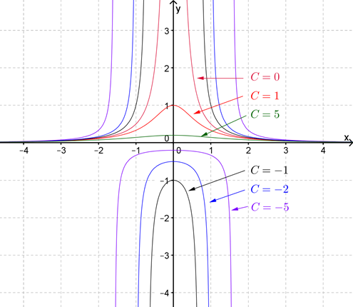
\begin{equation*} y(x)=\frac{1}{2x^2+C}, \hspace{5mm} y(x)=0 \hspace{5mm} \textrm{ for } C\in\mathbb{R} \end{equation*}

See Figure 10.5 for a sketch of these solutions for various values of \(C\text{.}\)

Figure 10.5. A sketch of \(y(x)=\frac{1}{2x^2+C}\) for various values of \(C\text{.}\)

The Sage cell below can be used to plot the direction field of \(\dfrac{dy}{dx}\) as well as the solution \(y(x)\) for a given constant of integration \(c\text{.}\)

Example 10.6.

Find the solution to the initial-value problem

\begin{equation*} (4y-\cos(y))\frac{dy}{dt}-3t^2=0, \hspace{5mm} y(0)=0 \end{equation*}

Answer.

\(2y^2-\sin(y)=t^3\)

Solution.

This is a first order separable DE so begin by separating the variables, i.e.

\begin{equation*} (4y-\cos(y))\frac{dy}{dt}=3t^2 \end{equation*}

Integrating both sides with respect to \(t\) and applying the integration by substitution formula to the left hand side gives

\begin{equation*} \int 4y-\cos(y)\hspace{2mm} dy=\int 3t^2\hspace{2mm} dt \end{equation*}

Evaluating the integrals on both sides (and combining the two constants of integration) gives

\begin{equation*} 2y^2-\sin(y)=t^3+C \end{equation*}

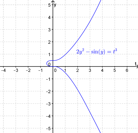
We can’t make \(y\) the subject of this equation and so in this case we can’t find an explicit formula for the general solution to the DE. Substituting the initial condition into the implicit equation gives

\begin{equation*} 2\times 0^2-\sin(0)=0^3+C \end{equation*}

i.e.

\begin{equation*} C=0 \end{equation*}

Thus the solution to the initial-value problem is the relevant function \(y(t)\) defined implicitly by

\begin{equation*} 2y^2-\sin(y)=t^3 \end{equation*}

The curve defined implicitly by this equation is shown in Figure 10.7 and from this we can see that the "bottom" part of the curve will be the function that is the solution to the initial-value problem.

The Sage cell below can be used to plot the direction field of \(\dfrac{dy}{dt}\) as well as the solution \(y(x)\) for a given constant of integration \(c\text{.}\)

Example 10.8.

Find the general solution to the DE

\begin{equation*} \frac{dy}{dx}=y(1-y) \end{equation*}

Note: We looked at this example in Chapter 9. There we sketched a direction field for the DE.

Answer.

\(y(x)=\dfrac{Ae^x}{1+Ae^x}\)

Solution.

This is a first order separable DE with \(f(x)=1\) (i.e. it is autonomous) and \(g(y)=y(1-y)\text{.}\) On separating the variables and integrating both sides with respect to \(x\) we obtain

\begin{equation*} \int \frac{1}{y(1-y)}\hspace{2mm}dy=\int 1\hspace{2mm}dx \end{equation*}

To evaluate the integral on the left hand side we have to use partial fraction decomposition, by which we can determine that

\begin{equation*} \frac{1}{y(1-y)}=\frac{1}{y}+\frac{1}{1-y} \end{equation*}

Thus

\begin{align*} \int \frac{1}{y(1-y)}\hspace{2mm}dy \amp=\int \frac{1}{y}\hspace{2mm}dy +\int \frac{1}{1-y}\hspace{2mm}dy\\ \amp =\ln(\vert y\vert)-\ln(\vert 1-y\vert)+C \end{align*}

(Some more detail on partial fraction decomposition can be found in an appendix to this lecture.) So, on evaluating the integral on the right hand side and combining the two constants of integration we obtain

\begin{equation*} \ln(\vert y\vert)-\ln(\vert 1-y\vert)=x+K \end{equation*}

This can be rearranged as

\begin{equation*} y(x)=\frac{Ae^x}{1+Ae^x} \end{equation*}

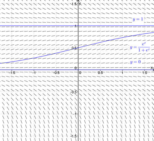
Figure 10.9 shows this curve when \(A=1\) superimposed on top of the direction field for the DE. Also shown in the figure are the solutions \(y(x)=0\) and \(y(x)=1\) which come from checking separately the cases where \(g(y)=0\text{.}\)

The Sage cell below can be used to plot the direction field of \(\dfrac{dy}{dx}\) as well as the solution \(y(x)\) for a given constant of integration \(A\text{.}\)

Example 10.10.

Find the solution to the initial-value problem

\begin{equation*} \frac{dy}{dx}=xy+x, \hspace{5mm} y(0)=1 \end{equation*}

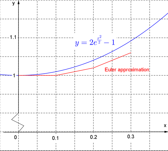
Note: We looked at this example in section Chapter 9 where we used Euler’s method with \(\Delta x=0.1\) to approximate the value of the solution at \(x=0.3\text{.}\)

Answer.

\(y(x)=2e^{x^2/2}-1\)

Solution.

This is a first order separable DE with \(f(x)=x\) and \(g(y)=y+1\text{.}\) On separating the variables and integrating both sides with respect to \(x\) we obtain

\begin{equation*} \int \frac{1}{y+1}\hspace{2mm}dy=\int x\hspace{2mm}dx \end{equation*}

Evaluating the integrals and rearranging gives

\begin{equation*} y(x)=Ce^{x^2/2}-1 \end{equation*}

To satisfy the initial condition

\begin{align*} 1 \amp=Ce^0-1\\ C \amp =2 \end{align*}

Thus the solution to the initial-value problem is

\begin{equation*} y(x)=2e^{x^2/2}-1 \end{equation*}

Note: From this solution

\begin{equation*} y(0.3)=2e^{(0.3)^2/2}-1=1.0921 \textrm{ to 4.d.p.} \end{equation*}

The Euler method approximation was

\begin{equation*} y(0.3)=1.0604 \textrm{ to 4.d.p.} \end{equation*}

Figure 10.11 shows both the analytic solution and the Euler approximation over the domain \(0\leq x\leq 0.3\text{.}\)

Figure 10.11. Plot of the analytic solution (blue) and Euler approximation (red) for \(\frac{dy}{dx}=xy+x\text{.}\)

Exercises Example Tasks

1.

Find the general solution to the DE

\begin{equation*} \frac{\sqrt{1+x^2}}{y+1}\frac{dy}{dx}=-x \end{equation*}

2.

Solve the initial-value problem

\begin{equation*} y'=-\frac{x}{y+1}, \hspace{5mm} y(0)=2 \end{equation*}

Section 10.2 Some Simple Applications of First Order Separable DEs

Example 10.12.

Find a curve in the \(xy\)-plane that passes through the point \((0,3)\) and whose tangent line at any point \((x,y)\) has its slope given by \(\frac{2x}{y^2}\text{.}\)

Answer.

\(y(x)=(3x^2+27)^{1/3}\)

Solution.

Let the curve be \(y(x)\text{.}\) Then we know

\begin{equation*} y'=\frac{2x}{y^2}, \hspace{5mm} y(0)=3 \end{equation*}

i.e. \(y\) is the solution to an initial-value problem involving a first order separable DE. From the DE, we obtain

\begin{equation*} \int y^2 \hspace{2mm}dy=\int 2x\hspace{2mm}dx \end{equation*}

and hence

\begin{equation*} \frac{1}{3}y^3=x^2+C \end{equation*}

Using the initial condition gives \(C=9\) and hence the required curve is

\begin{equation*} y(x)=(3x^2+27)^{1/3} \end{equation*}

Example 10.13.

Suppose that the temperature a cup of coffee when it is poured is \(95^oC\text{.}\) The cup is left to stand in a room where the temperature is \(20^oC\text{.}\) If the temperature of the coffee is \(90^oC\) after \(2\) min, how long will it take for the temperature of the coffee in the cup to reach \(25^oC\) according to Newton’s law of cooling?

Answer.

\(t\approx 78.5 \textrm{ min}\)

Solution.

Let \(T(t)\) be the temperature of the cup of coffee at time \(t\) min after it was poured and let \(T_a\) be the room (ambient) temperature. Now, Newton’s law of cooling says that the rate at which the temperature of an object falls is proportional to the difference in the temperature of the object and the temperature of its surroundings. Thus

\begin{equation*} \frac{dT}{dt}=-k(T-T_a), \hspace{5mm} T(0)=95, \hspace{5mm} T(2)=90 \end{equation*}

where \(k\gt 0\) is the constant of proportionality. This is a first order separable DE and on separating the variables and integrating both sides with respect to \(t\) we get

\begin{equation*} \int \frac{1}{T-T_a}\hspace{2mm}dT=\int -k\hspace{2mm}dt \end{equation*}

Evaluating the integrals gives

\begin{align*} \ln(\vert T-T_a\vert) \amp=-kt+C\\ T(t) \amp =Ae^{-kt}+T_a \end{align*}

Since \(T_a=20\text{,}\) using \(T(0)=95\) gives \(A=75\text{.}\) Using \(T(2)=90\) gives

\begin{equation*} 90=75e^{-2k}+20 \end{equation*}

and hence

\begin{equation*} k=-\frac{\ln(\frac{14}{15})}{2}\approx 0.034 \end{equation*}

Thus, according to Newton’s law of cooling the coffee will have cooled to \(25^oC\) at the value of \(t\) satisfying

\begin{equation*} 25=75e^{-kt}+20 \end{equation*}

from which we find

\begin{equation*} t=-\frac{\ln(\frac{1}{15})}{k}\approx 78.5 \textrm{ min} \end{equation*}

Example 10.14.

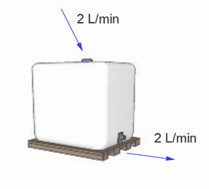
Consider a \(100\)L tank which contains pure water. At time \(t=0\) salt water begins to flow into the tank at a rate of \(2\)L/min and the mixed water flows out of the tank at the same rate. If the concentration of the salt in the inflowing water is \(35\)g/L determine the concentration, \(C(t)\text{,}\) of the salt in the tank as a function of time.

Figure 10.15. Flow of water in and out of a tank.

Answer.

\(C(t)=35-35e^{-t/50}\)

Solution.

Let \(A(t)\) be the amount of salt in the tank (in grams) at time \(t\text{.}\) Then, since there is \(100\)L of water in the tank

\begin{equation} A(t)=100\times C(t)\tag{10.1} \end{equation}

Now, since the water in the tank is initially pure, we have the initial condition \(A(0)=0\) or equivalently \(C(0)=0\text{.}\) Finally, the rate at which the amount of salt in the tank is changing is given by the difference of the rate at which the amount of salt is increasing (due to the salt water entering the tank) and the rate at which the amount is decreasing (due to the mixed water flowing out). Since salt water is entering the tank at a rate of \(2\)L/min and each litre contains \(35\)g of salt, the rate at which the amount of salt is increasing is \(70\)g/min. Since the mixed water is flowing out of the tank at the rate of \(2\)L/min and each litre contains \(C(t)\)g the rate at which the amount of salt is decreasing is \(2C\)g/min. Thus

\begin{equation} \frac{dA}{dt}=70-2C\tag{10.2} \end{equation}

From (10.1),

\begin{equation} \frac{dA}{dt}=100\frac{dC}{dt}\tag{10.3} \end{equation}

Putting (10.3) into (10.2),

\begin{equation*} 100\frac{dC}{dt}=70-2C \end{equation*}

which is a first order separable DE. Separating the variables and integrating both sides with respect \(t\) gives

\begin{equation*} \int \frac{1}{70-2C}\hspace{2mm} dC=\int \frac{1}{100}\hspace{2mm}dt \end{equation*}

Evaluating the integrals gives

\begin{equation*} -\frac{1}{2}\ln(70-2C)=\frac{1}{100}t+K \end{equation*}

and hence

\begin{equation*} C(t)=35-ke^{-t/50} \end{equation*}

Using the initial condition \(C(0)=0\) gives \(k=35\) and hence

\begin{equation*} C(t)=35-35e^{-t/50} \end{equation*}

Exercises Example Tasks

1.

An ingot of gold is placed into a furnace which has a temperature of \(1200^oC\text{.}\) After \(3\) min the temperature of the ingot has risen from \(40^oC\) to \(610^oC\text{.}\) Assuming Newton’s Law of Cooling how long before the ingot reaches the melting temperature of \(1064^oC\text{?}\)

2.

Consider a \(50\)L tank which contains salt water with concentration of \(20\)g/L. At time \(t=0\) more salt water begins to flow into the tank at the rate of \(3\)L/min and the mixed water flows out of the tank at the same rate. Assuming that the concentration of salt in the inflowing water is \(30\)g/L how long will it take for the concentration of the water in the tank to reach \(25\)g/L?

Appendix 10.A Partial Fraction Decomposition

Partial fraction decomposition is, essentially, the inverse operation of combining fractions by putting them over a common denominator. More formally, partial fraction decomposition expresses a proper rational function (i.e. a function that is the ratio of two polynomials where the degree of the polynomial in the denominator is greater that the degree of the polynomial in the numerator) as the sum of proper rational functions of lesser degree.

Example 10.16.

Write \(\dfrac{2}{x+2}-\dfrac{3}{2x-1}\) as a single fraction.

Answer.

\(=\dfrac{x-8}{(x+2)(2x-1)}\)

Solution.

Using \((x+2)(2x-1)\) as the common denominator we get

\begin{align*} \frac{2}{x+2}-\frac{3}{2x-1} \amp=\frac{2(2x-1)}{(x+2)(2x-1)}-\frac{3(x+2)}{(x+2)(2x-1)}\\ \amp =\frac{4x-2-3x-6}{(x+2)(2x-1)}\\ \amp =\frac{x-8}{(x+2)(2x-1)} \end{align*}

In partial fraction decomposition, for each distinct linear factor \((ax+b)\) in the denominator include a term \(\dfrac{A}{ax+b}\) in the decomposition, where \(A\) is a value we have to determine.

Example 10.17.

Find the partial fraction decomposition of \(\dfrac{x-8}{(x+2)(2x-1)}\text{.}\)

Answer.

\(\dfrac{x-8}{(x+2)(2x-1)}=\dfrac{2}{x+2}-\dfrac{3}{2x-1}\)

Solution.

Because the denominator of this rational function contains two linear polynomial terms the partial fraction decomposition takes the form

\begin{equation} \frac{x-8}{(x+2)(2x-1)}=\frac{A}{x+2}+\frac{B}{2x-1}\tag{10.4} \end{equation}

To determine the values for \(A\) and \(B\) multiply both sides of (10.4) by \((x+2)(2x-1)\text{.}\) This gives

\begin{align*} x-8 \amp=A(2x-1)+B(x+2)\\ \amp =(2A+B)x+(2B-A) \end{align*}

For the polynomials on both sides of the equation to be equal they must have the same coefficients and so

\begin{align*} 2A+B \amp=1\\ -A+2B \amp=-8 \end{align*}

Solving these simultaneous equations gives \(A=2,\hspace{2mm} B=-3\) and hence

\begin{equation*} \frac{x-8}{(x+2)(2x-1)}=\frac{2}{x+2}-\frac{3}{2x-1} \end{equation*}

If the denominator of the rational function contains a linear factor to some power, i.e. \((ax+b)^n\text{,}\) then the partial fraction decomposition should contain the terms

\begin{equation*} \frac{A_1}{ax+b}+\frac{A_2}{(ax+b)^2}+...+\frac{A_n}{(ax+b)^n} \end{equation*}

If the denominator of the rational function contains a quadratic factor, i.e. \((ax^2+bx+c)\text{,}\) then the partial fraction decomposition should contain the term

\begin{equation*} \frac{Ax+B}{ax^2+bx+c} \end{equation*}

Example 10.18.

Find the partial fraction decomposition of \(\dfrac{2x^3-5x^2+2x-2}{(x^2+2)(x-1)^2}\text{.}\)

Answer.

\(\dfrac{2x^3-5x^2+2x-2}{(x^2+2)(x-1)^2}=\dfrac{2x}{x^2+2}-\dfrac{1}{(x-1)^2}\)

Solution.

Because the denominator contains a quadratic term a repeated linear term the partial fraction decomposition takes the form

\begin{equation} \frac{2x^3-5x^2+2x-2}{(x^2+2)(x-1)^2}=\frac{Ax+B}{x^2+2}+\frac{C}{x-1}+\frac{D}{(x-1)^2}\tag{10.5} \end{equation}

Multiply both sides of (10.5) by \((x^2+2)(x-1)^2\) and collect like terms. This gives

\begin{equation*} 2x^3-5x^2+2x-2=(A+C)x^3+(-2A+B-C+D)x^2+(A-2B+2C)x+(B-2C+2D) \end{equation*}

Equating the coefficients of the polynomials on each side gives

\begin{align*} A+C \amp =2\\ -2A+B-C+D \amp=-5\\ A-2B+2C \amp =2\\ B-2C+2D \amp=-2 \end{align*}

Solving these simultaneous equations gives \(A=2\text{,}\) \(B=0\text{,}\) \(C=0\text{,}\) \(D=-1\) and hence

\begin{equation*} \frac{2x^3-5x^2+2x-2}{(x^2+2)(x-1)^2}=\frac{2x}{x^2+2}-\frac{1}{(x-1)^2} \end{equation*}

Exercises Example Tasks

1.

Evaluate the integral

\begin{equation*} \int \frac{x^2-2x+3}{(x^2+1)(x-1)}\hspace{2mm} dx \end{equation*}

Prev Top Next