LA3: Matrix Algebra

Chapter 17 LA3: Matrix Algebra

We introduced matrices when discussing systems of linear equations. Recall that an \(m \times n\) matrix is a rectangular array of numbers, written in the form

\begin{equation*} \begin{pmatrix} a_{11} \amp a_{12} \amp \cdots \amp a_{1n}\\ a_{21} \amp a_{22} \amp \cdots \amp a_{2n}\\ \vdots \amp \vdots \amp \ddots \amp \vdots\\ a_{m1} \amp a_{m2} \amp \cdots \amp a_{mn}\\ \end{pmatrix}, \end{equation*}

which is sometimes written in the abbreviated form

\begin{equation*} A=\left(a_{ij}\right)_{m \times n}. \end{equation*}

Note that we usually use a capital letter to denote a matrix.

In the context of systems of linear equations the main concept was row reducing a matrix to produce equivalent matrices. In different contexts, however, other operations on matrices have proved useful and we shall discuss these operations below. Before doing this, though, we will introduce some new terminology.

Definition 17.1.

Two matrices are said to be equal if they are of the same size and all corresponding entries are equal.

Example 17.2.

Let \(A = \begin{pmatrix}5 \amp 0 \amp 1\\ -3 \amp \sqrt{2} \amp \frac{1}{2}\end{pmatrix}, \quad B = \begin{pmatrix}5 \amp -3 \\ 0 \amp \sqrt{2} \\ 1 \amp \frac{1}{2}\end{pmatrix}, \quad C = \begin{pmatrix} 5 \amp 0 \amp 1\\ -3 \amp a \amp b\end{pmatrix}.\)

For what values of \(a\) and \(b\) does \(A=C\text{?}\)
For what values of \(a\) and \(b\) does \(B=C\text{?}\)

Answer.

\(a=\sqrt{2}\) and \(b=\dfrac{1}{2}\)
None.

Solution.

Since \(A\) and \(C\) are of the same size, the matrices will be equal when \(a=\sqrt{2}\) and \(b=\dfrac{1}{2}\text{.}\)
Since \(B\) and \(C\) are not the same size they can never be equal.

Definition 17.3.

The zero \(m \times n\) matrix is the \(m \times n\) matrix with all entries \(0\text{,}\) i.e.

\begin{equation*} 0 = \begin{pmatrix} 0 \amp 0 \amp \cdots \amp 0\\ 0 \amp 0\amp \cdots \amp 0\\ \vdots \amp \vdots \amp \ddots \amp \vdots\\ 0\amp 0\amp \cdots \amp 0\\ \end{pmatrix}. \end{equation*}

Note that by using the symbol \(0\) to denote the zero matrix we have to tell from the context whether the \(0\) refers to a number or a matrix.

Definition 17.4.

For the matrix \(A=(a_{ij})_{m \times n}\text{,}\) its transpose, denoted by \(A^T\text{,}\) is defined by \(A^T = \left(a_{ji}\right)_{n \times m}\text{.}\)

Note that this definition is saying that the rows of matrix \(A\) are the columns of its transpose \(A^T\) and vice versa.

Example 17.5.

Let

\begin{equation*} B = \begin{pmatrix}5 \amp -3 \\ 0 \amp \sqrt{2} \\ 1 \amp \frac{1}{2}\end{pmatrix}, \quad C = \begin{pmatrix} 5 \amp 0 \amp 1\\ -3 \amp a \amp b\end{pmatrix}. \end{equation*}

For what values of \(a\) and \(b\) does \(B^T=C\text{?}\)

Answer.

\(a=\sqrt{2}, \ b=\dfrac{1}{2}\)

Solution.

Since \(B^T = \begin{pmatrix} 5 \amp 0 \amp 1\\ -3 \amp \sqrt{2} \amp \frac{1}{2}\end{pmatrix}\text{,}\) \(B^T = C\) when \(a=\sqrt{2}\) and \(b=\frac{1}{2}\text{.}\)

Definition 17.6.

A square matrix is a matrix that has the same number of rows and columns.

Example 17.7.

Matrix \(A\) is a square matrix whereas matrix \(B\) is not.

\begin{equation*} A = \begin{pmatrix}-1 \amp 3 \amp 4\\ 5 \amp 0 \amp -2 \\ 3 \amp \frac{1}{3} \amp 6 \end{pmatrix}, \quad B = \begin{pmatrix} -1 \amp 3 \\ 5 \amp 0 \\ 3 \amp \frac{1}{3}\end{pmatrix} \end{equation*}

Definition 17.8.

The \(n \times n\) identity matrix, \(I_n\), is the matrix with \(n\) rows and \(n\) columns with all entries on the main diagonal equal to \(1\) and all other entries \(0\text{,}\) i.e.

\begin{equation*} I_n = \begin{pmatrix} 1 \amp 0 \amp \cdots \amp 0\\ 0 \amp 1 \amp \cdots \amp 0\\ \vdots \amp \vdots \amp \ddots \amp \vdots\\ 0\amp 0 \amp \cdots \amp 1\ \end{pmatrix}. \end{equation*}

Often, when the size of the identity matrix is clear the subscript is dropped from the notation and the identity matrix is denoted just by \(I\text{.}\)

Section 17.1 Addition and Scalar Multiplication

Definition 17.9. Matrix addition and scalar multiplication.

Let \(A\) and \(B\) be \(m \times n\) matrices, i.e., \(A=\left(a_{ij}\right)_{m \times n}\) and \(B = \left(b_{ij}\right)_{m \times n}\text{.}\) Then

Matrix addition is defined by \(A+B = \left(a_{ij} + b_{ij}\right)_{m \times n}\text{.}\)
Scalar multiplication is defined by \(kA = \left(k \cdot a_{ij}\right)_{m \times n}\) where \(k\) is a constant.

Thus, to add two matrices of the same size, add up the corresponding entries in each matrix. Matrix addition of matrices not of the same size is not defined. To multiply a matrix by a scalar, multiply each entry in the matrix by that scalar. Note that we now can also subtract two matrices by defining

\begin{equation*} A-B = A+ (-1)B. \end{equation*}

Example 17.10.

If \(A = \begin{pmatrix} 1 \amp 2 \amp 3\\ 4 \amp 3 \amp 2\end{pmatrix}, \quad B = \begin{pmatrix} 5 \amp 3 \\ 9 \amp 2 \\ 4 \amp 3\end{pmatrix}.\) Then calculate the given expression or explain why it does not exist.

\(\displaystyle 3A+B\)
\((2A^T - B)_{32} \, \) (i.e. the entry in row \(3\text{,}\) column \(2\) of the matrix \(2A^T-B\,\))
\(\displaystyle (B^T+A)_{31}\)

Solution.

Since \(A\) is a \(2 \times 3\) matrix so will be \(3A\text{.}\) Since \(3A\) and \(B\) are not the same size we cannot add these two matrices.
\(A^T = \begin{pmatrix} 1 \amp 4 \\ 2 \amp 3 \\ 3\amp 2\end{pmatrix}\) and so \(2A^T = \begin{pmatrix} 2 \amp 8 \\ 4 \amp 6 \\ 6 \amp 4\end{pmatrix}\text{.}\) Thus \(2A^T-B = \begin{pmatrix} -3 \amp 5 \\ -5 \amp 4 \\ 2 \amp 1\end{pmatrix}\) and \((2A^T - B)_{32} =1.\)
\(B^T + A = \begin{pmatrix} 5 \amp 9 \amp 4 \\ 3 \amp 2 \amp 3\end{pmatrix} + \begin{pmatrix} 1 \amp 2 \amp 3\\ 4 \amp 3 \amp 2\end{pmatrix} = \begin{pmatrix} 6 \amp 11 \amp 7\\ 7 \amp 5 \amp 5\end{pmatrix}\text{.}\) Since this is a \(2 \times 3\) matrix there is no entry in row \(3\text{,}\) column \(1\text{.}\)

From the definitions of matrix addition and scalar multiplication the following general properties can be shown.

Theorem 17.11. Properties of Scalar Multiplication and Matrix Addition.

Let \(A\text{,}\) \(B\) and \(C\) be matrices of the same size. Then

(A1): \(A+B = B+A \hspace{32mm}\) (Commutative Law)
(A2): \((A+B)+C = A+(B+C) \hspace{10mm}\)(Associative Law)
(A3): \(A+0 = A \hspace{57mm}\) (Identity Law)
(A4): \(A+(-A) = 0 \hspace{50mm}\) (Inverse Law)
(S1): \(k(A+B) = kA+kB\)
(S2): \((k_1 + k_2)A= k_1A + k_2A\)
(S3): \(k_1(k_2A) = (k_1k_2)A\)
(S4): \(1A = A\)

Exercises Example Tasks

1.

Let

\begin{equation*} A = \begin{pmatrix}4 \amp -2 \amp 1\\ 0 \amp 2 \amp 3\end{pmatrix} \quad \mbox{and} \quad B=\begin{pmatrix}1 \amp 2 \\ 3 \amp 4 \\ 5 \amp 6\end{pmatrix}. \end{equation*}

Find \((2A-B^{T})_{12}\text{.}\)
Find \((2A-B)^T\text{.}\)

2.

Show that for any matrix \(A\,\text{,}\) \(3A = A + A + A\text{.}\) For what values of \(k\) is it true that \(kA = \underbrace{A + A + \cdots + A}_{k \mbox{ times}}\,\text{?}\)

3.

Prove that for two matrices \(A\) and \(B\) of the same size \(A+B = B+A\text{.}\)

Section 17.2 Matrix Multiplication

Definition 17.12.

Let \(A=\left(a_{ij}\right)_{m \times n}\) and \(B = \left(b_{ij}\right)_{n \times p}\text{.}\) Then matrix multiplication is defined by

\begin{equation*} AB = \left(\sum_{k=1}^n a_{ik}b_{kj}\right)_{m \times p}. \end{equation*}

If we call \(C=AB\) then from this definition it can be seen:

For the matrix multiplication \(AB\) to be defined the number of columns in \(A\) has to be equal to the number of rows in \(B\text{.}\) The resulting matrix, \(C\text{,}\) has the same number of rows as \(A\) and the same number of columns as \(B\text{.}\)
Entry \(c_{ij}\) in \(C\) is found by taking the scalar (or dot) product of the \(i^{\mbox{th}}\) row vector from \(A\) with (the transpose of) the \(j^{\mbox{th}}\) column vector from \(B\text{,}\) i.e.
\begin{align*} c_{ij} \amp = (a_{i1},a_{i2}, \ldots, a_{in})\cdot (b_{1j},b_{2j}, \ldots, b_{nj}) \\ \amp = a_{i1}b_{1j} + a_{i2}b_{2j} + \cdots + a_{in}b_{nj}. \end{align*}

Example 17.13.

Let

\begin{equation*} A=\begin{pmatrix} 0 \amp 1 \\ -1 \amp 3 \\ 2 \amp 5 \end{pmatrix} \quad \mbox{and} \quad B=\begin{pmatrix} -2 \amp 1/2 \\ -3 \amp 4 \end{pmatrix}. \end{equation*}

Calculate \(AB\text{.}\)
Calculate \(BA\text{.}\)

Answer.

\(\displaystyle AB=\begin{pmatrix} -3 \amp 4 \\ -7 \amp 23/2 \\ -19 \amp 21 \end{pmatrix}\)
\(BA\) is not defined.

Solution.

Since \(A\) is a \(3 \times 2\) matrix and \(B\) is \(2\times 2\) then \(AB\) is defined since \(A\) has \(2\) columns and \(B\) has \(2\) rows. The resultant matrix will be a \(3 \times 2\) matrix since \(A\) has \(3\) rows and \(B\) has \(2\) columns. Thus \(AB\) will be of the form

\begin{equation*} AB = \begin{pmatrix}c_{11} \amp c_{12}\\ c_{21} \amp c_{22}\\ c_{31} \amp c_{32}\end{pmatrix}. \end{equation*}

Now

\begin{align*} c_{11} \amp = (0,1)\cdot (-2,-3) = 0 -3 = -3 \\ c_{12} \amp = (0,1)\cdot (1/2,4) = 0 + 4 = 4 \\ c_{21} \amp = (-1,3)\cdot (-2,-3) = 2 - 9 = -7 \\ c_{22} \amp = (-1,3)\cdot (1/2,4) = -1/2 +12 = 23/2 \\ c_{31} \amp = (2,5)\cdot (-2,-3) = -4 -15 = -19 \\ c_{32} \amp = (2,5)\cdot (1/2,4) = 1 + 20 = 21 \end{align*}

and so

\begin{equation*} AB=\begin{pmatrix} -3 \amp 4 \\ -7 \amp 23/2 \\ -19 \amp 21 \end{pmatrix}. \end{equation*}
\(BA\) is not defined because the number of columns in \(B\) (i.e. 2) is not equal to the number of rows in \(A\) (i.e. 3).

Notice that this example shows that matrix multiplication is not commutative, i.e. in general

\begin{equation*} AB \neq BA. \end{equation*}

Example 17.14.

Let

\begin{equation*} A=\begin{pmatrix} 3\amp 2 \amp 1 \amp 6 \\ 2 \amp 1 \amp 3 \amp -1\end{pmatrix}, \quad B=\begin{pmatrix} 1 \amp 0 \\ -1 \amp 2 \\ 3 \amp 1 \\ 4 \amp 5 \end{pmatrix}, \quad C =\begin{pmatrix}-2 \amp 1 \amp 0 \\ 4 \amp -1 \amp 3\end{pmatrix}. \end{equation*}

Calculate \(A(BC)\text{.}\)
Calculate \((AB)C\text{.}\)

Answer.

\(A(BC) = \begin{pmatrix}84 \amp -7 \amp 105 \\ -12 \amp 6 \amp 0\end{pmatrix} = (AB)C\)

Solution.

\(BC = \begin{pmatrix} 1 \amp 0 \\ -1 \amp 2 \\ 3 \amp 1 \\ 4 \amp 5 \end{pmatrix}\begin{pmatrix}-2 \amp 1 \amp 0 \\ 4 \amp -1 \amp 3\end{pmatrix} = \begin{pmatrix} -2 \amp 1 \amp 0\\ 10 \amp -3 \amp 6 \\ -2 \amp 2 \amp 3 \\ 12 \amp -1 \amp 15\end{pmatrix}\)

\begin{equation*} A(BC) = \begin{pmatrix} 3\amp 2 \amp 1 \amp 6 \\ 2 \amp 1 \amp 3 \amp -1\end{pmatrix}\begin{pmatrix} -2 \amp 1 \amp 0\\ 10 \amp -3 \amp 6 \\ -2 \amp 2 \amp 3 \\ 12 \amp -1 \amp 15\end{pmatrix} = \begin{pmatrix} 84 \amp -7 \amp 105 \\ -12 \amp 6 \amp 0\end{pmatrix}. \end{equation*}
\(AB = \begin{pmatrix} 3\amp 2 \amp 1 \amp 6 \\ 2 \amp 1 \amp 3 \amp -1\end{pmatrix} \begin{pmatrix} 1 \amp 0 \\ -1 \amp 2 \\ 3 \amp 1 \\ 4 \amp 5 \end{pmatrix} = \begin{pmatrix} 28 \amp 35 \\ 6 \amp 0\end{pmatrix}\)

\begin{equation*} (AB)C = \begin{pmatrix} 28 \amp 35 \\ 6 \amp 0\end{pmatrix} \begin{pmatrix}-2 \amp 1 \amp 0 \\ 4 \amp -1 \amp 3\end{pmatrix} = \begin{pmatrix}84 \amp -7 \amp 105 \\ -12 \amp 6 \amp 0\end{pmatrix}. \end{equation*}

Notice that this example is an illustration that matrix multiplication is associative, i.e. in general

\begin{equation*} A(BC) = (AB)C\text{.} \end{equation*}

From the definition of matrix multiplication the following properties can be shown to hold.

Theorem 17.15. Properties of Matrix Multiplication.

Let \(A\text{,}\) \(B\) and \(C\) be appropriately sized matrices. Then

\(A(BC)=(AB)C \hspace{55mm}\) (Associative Law)
\(A(B+C) = AB + AC \hspace{42mm}\) (Left Distributive Law)
\((A+B)C = AC + BC \hspace{42mm}\) (Right Distributive Law)
\(\displaystyle k(AB) = (kA)B = A(kB)\)
\(I_mA = A = AI_n\) if \(A\) is an \(m \times n\) matrix\(\hspace{5mm}\) (Identity Law)

For later reference, some properties of the transpose of a matrix with respect to the various matrix operations that we have been discussing are listed below.

Theorem 17.16. Properties of Matrix Transpose.

Let \(A\) and \(B\) be appropriately sized matrices. Then

\(\displaystyle (A^T)^T = A\)
\(\displaystyle (A+B)^T = A^T + B^T \)
\(\displaystyle (kA)^T = k(A^T) \)
\(\displaystyle (AB)^T = B^TA^T \)
\((A^r)^T = (A^T)^r \) where \(r \in \mathbb{N}\text{.}\)

Example 17.17.

Confirm that \((AB)^T = B^T A^T\) holds for the matrices

\begin{equation*} A = \begin{pmatrix}0 \amp 1\\ -1 \amp 3 \\ 2 \amp 5\end{pmatrix} \quad \mbox{and} \quad B = \begin{pmatrix}-2 \amp 1/2 \\ -3 \amp 4 \end{pmatrix}. \end{equation*}

Solution.

Firstly

\begin{align*} (AB)^T \amp = \left( \begin{pmatrix}0 \amp 1\\ -1 \amp 3 \\ 2 \amp 5\end{pmatrix} \begin{pmatrix}-2 \amp 1/2 \\ -3 \amp 4 \end{pmatrix}\right)^T\\ \amp = \begin{pmatrix}-3 \amp 4 \\ -7 \amp 23/2 \\ -19 \amp 21\end{pmatrix}^T\\ \amp = \begin{pmatrix}-3 \amp -7 \amp -19 \\ 4 \amp 23/2 \amp 21 \end{pmatrix}. \end{align*}

\begin{align*} B^TA^T \amp = \begin{pmatrix}-2 \amp -3 \\ 1/2 \amp 4 \end{pmatrix} \begin{pmatrix}0 \amp -1 \amp 2\\ 1 \amp 3 \amp 5\end{pmatrix} \\ \amp = \begin{pmatrix}-3 \amp -7 \amp -19 \\ 4 \amp 23/2 \amp 21 \end{pmatrix}. \end{align*}

Exercises Example Tasks

1.

Let

\begin{equation*} A = \begin{pmatrix} 3 \amp -1 \\ -2 \amp 2\end{pmatrix} \quad \mbox{ and } \quad B=\begin{pmatrix} 0 \amp 1 \\ 4 \amp -1 \end{pmatrix}. \end{equation*}

Calculate \((A+B)^2\text{.}\)
Calculate \(A^2 + 2AB + B^2\text{.}\)

2.

Let

\begin{equation*} E = \begin{pmatrix} 6 \amp 1 \\ -1 \amp 3 \\ -5 \amp 2\end{pmatrix} \quad \mbox{ and } \quad F=\begin{pmatrix} 1 \amp -2 \amp 0 \\ 3 \amp 1 \amp 4 \end{pmatrix}. \end{equation*}

Calculate \((EF)_{23}\text{.}\)
Calculate \((FE)_{12}\text{.}\)

Section 17.3 Matrices and Systems of Linear Equations

Consider the following system of linear equations

\begin{align*} a_{11}x_1 + a_{12}x_2 + \cdots + a_{1n}x_n \amp= b_1\\ a_{21}x_1 + a_{22}x_2 + \cdots + a_{2n}x_n \amp= b_2\\ \quad\amp \vdots \quad\\ a_{m1}x_1 + a_{m2}x_2 + \cdots + a_{mn}x_n \amp= b_m \end{align*}

Now that we have introduced matrix multiplication we can write this system as

\begin{equation*} A \mathbf{x} = \mathbf{b} \end{equation*}

where \(A\) is the \(m \times n\) coefficient matrix

\begin{equation*} A = \begin{pmatrix} a_{11} \amp a_{12} \amp \cdots \amp a_{1n}\\ a_{21} \amp a_{22} \amp \cdots \amp a_{2n}\\ \vdots \amp \vdots \amp \ddots \amp \vdots\\ a_{m1} \amp a_{m2} \amp \cdots \amp a_{mn}\\ \end{pmatrix}, \end{equation*}

\(\mathbf{x}\) is the \(n \times 1\) matrix (i.e. the column vector of the variables)

\begin{equation*} \mathbf{x}=\begin{pmatrix}x_1 \\ x_2 \\\vdots \\x_n\end{pmatrix} \end{equation*}

and \(\mathbf{b}\) is the \(m \times 1\) (i.e. the column vector of the constants)

\begin{equation*} \mathbf{b} = \begin{pmatrix}b_1 \\ b_2 \\ \vdots \\ b_m\end{pmatrix}. \end{equation*}

Example 17.18.

The system of linear equations

\begin{align*} 3x_1 - x_2 + 2x_3 + x_4 \amp= 2\\ -x_1 + 6x_2 - 11x_4 \amp= -22\\ x_1 + x_2 + 7x_3 + 4x_4 \amp= 8 \end{align*}

can be written as

\begin{equation*} A = \begin{pmatrix} 3 \amp -1 \amp 2 \amp 1 \\ -1 \amp 6 \amp 0 \amp -11 \\ 1 \amp 1 \amp 7 \amp 4 \end{pmatrix} \begin{pmatrix}x_1\\ x_2 \\ x_3 \\ x_4\end{pmatrix} = \begin{pmatrix} 2 \\ -22 \\ 8\end{pmatrix}. \end{equation*}

We can now use the properties of matrix multiplication to establish some interesting facts about the solutions to systems of linear equations. For example:

Theorem 17.19.

Consider the non-homogenous system of linear equations

\begin{equation} A\mathbf{x} = \mathbf{b}, \ \mathbf{b} \neq 0\tag{17.1} \end{equation}

and the corresponding homogeneous system

\begin{equation} A\mathbf{x} = \mathbf{0}\tag{17.2} \end{equation}

If (17.1) has two distinct solutions then it has an infinite number of solutions.
If (17.1) has a unique solution then (17.2) has only the trivial solution \(\mathbf{x}=\mathbf{0}\text{.}\)
If (17.1) has an infinite number of solution then so does (17.2).

Proof.

Let \(\mathbf{x} = \mathbf{u}\) and \(\mathbf{x} = \mathbf{v}\) be two distinct solutions to (17.1) and let \(\mathbf{w} = \mathbf{u} − \mathbf{v}\text{.}\) By using the properties of matrix multiplication we can see that

\begin{equation*} A\mathbf{w} = A(\mathbf{u} − \mathbf{v}) = A\mathbf{u} − A\mathbf{v} =\mathbf{b} − \mathbf{b} = \mathbf{0}. \end{equation*}

So, any vector of the form \(\mathbf{u} + t\mathbf{w}\text{,}\) \(t \in \mathbb{R}\text{,}\) will be a solution to (17.1) since

\begin{equation*} A(\mathbf{u} +t\mathbf{w}) = A\mathbf{u} + A(t\mathbf{w}) = A\mathbf{u} +tA\mathbf{w} = \mathbf{b} +t\mathbf{0} = \mathbf{b}\text{,} \end{equation*}

i.e. (17.1) has an infinite number of solutions.
Let \(\mathbf{x} = \mathbf{u}\) be the unique solution to (17.1) and let \(\mathbf{x} = \mathbf{v}\) be a non-zero solution to (17.2). Then

\begin{equation*} A(\mathbf{u} + \mathbf{v}) = A\mathbf{u} + A\mathbf{v} = \mathbf{b} + \mathbf{0} = \mathbf{b} \end{equation*}

and so \(\mathbf{x} = \mathbf{u} + \mathbf{v}\) is another solution to (17.1), which is not possible. Thus there cannot be any non-zero solutions to (17.2).
Since (17.1) has an infinite number of solutions let \(\mathbf{x} = \mathbf{u}\) and \(\mathbf{x} = \mathbf{v}\) be two distinct solutions to (17.1). Now let \(\mathbf{w} = \mathbf{u} − \mathbf{v}\) and \(t \in \mathbb{R}\text{.}\) Then
\begin{equation*} A(t\mathbf{w}) = tA(\mathbf{u} − \mathbf{v}) = t(A\mathbf{u} − A\mathbf{v}) = t(\mathbf{b} − \mathbf{b}) = \mathbf{0}\text{,} \end{equation*}
i.e. there are an infinite number of solutions to (17.2).

Note that these arguments are general and hold for any system of \(m\) linear equations in \(n\) variables. Note also that if the system consists of \(3\) linear equations in \(3\) variables then result (17.2) above can be stated as:

Remark 17.20.

Consider the system of linear equations whose augmented matrix is

\begin{equation*} \begin{pmatrix} a_{11} \amp a_{12} \amp a_{13} \amp b_1 \\ a_{21} \amp a_{22} \amp a_{23} \amp b_2 \\ a_{31} \amp a_{32} \amp a_{33} \amp b_3 \end{pmatrix}. \end{equation*}

The following statements are equivalent:

The system has a unique solution.
The planes represented by the rows intersect in a point.
The column vectors of the coefficient matrix are linearly independent.

Exercises Example Tasks

1.

Consider the following system of linear equations:

\begin{align*} x_1 -x_2 -x_3 \amp =1\\ x_2 + 3x_3 \amp =1\\ 2x_1 -x_2 +x_3 \amp =3. \end{align*}

Calculate \(A\mathbf{u}\) where
\begin{equation*} A=\begin{pmatrix}1 \amp -1 \amp -1 \\ 0 \amp 1 \amp 3 \\ 2 \amp -1 \amp 1\end{pmatrix}, \quad \mathbf{u} = \begin{pmatrix}2 \\ 3 \\ -1\end{pmatrix}\text{.} \end{equation*}
Show that \((1,1,0)\) is a solution to the system of equations.
Write down all solutions to the system of equations.

Section 17.4 Linear Transformations

There are many applications of matrices where we view the matrix as a transformation (or mapping) that takes one vector and transforms (or maps) it to another vector. So, if \(A\) is an \(m \times n\) matrix then \(A\) can be thought of as a transformation that takes the \(n \times 1\) vector \(x\) to the \(m \times 1\) vector \(\mathbf{b} = A\mathbf{x}\text{.}\)

Example 17.21.

Consider the matrix

\begin{equation*} A = \begin{pmatrix} 0 \amp 1 \\ 1 \amp 0\end{pmatrix}. \end{equation*}

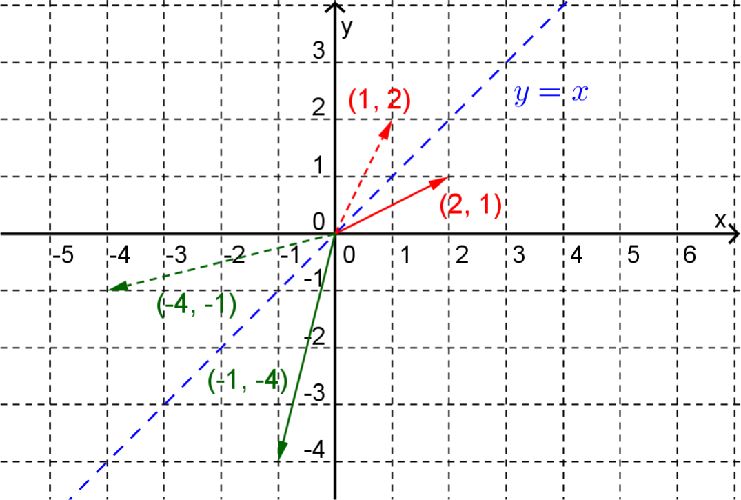
Since \(A\) is a \(2 \times 2\) matrix, we can think of \(A\) as a transformation that takes each vector \(x\) in the plane to another vector in the plane, \(b = A\mathbf{x}\text{.}\) Under this transformation, for example, \(\mathbf{x} = \begin{pmatrix} 2 \\ 1 \end{pmatrix}\) goes to

\begin{equation*} \mathbf{b} = A\mathbf{x} = \begin{pmatrix} 0 \amp 1 \\ 1 \amp 0\end{pmatrix}\begin{pmatrix}2 \\ 1\end{pmatrix} = \begin{pmatrix}1 \\ 2\end{pmatrix} \end{equation*}

and \(\mathbf{x} = \begin{pmatrix} -1 \\ -4\end{pmatrix}\) goes to

\begin{equation*} \mathbf{b} = A\mathbf{x} =\begin{pmatrix} 0 \amp 1 \\ 1 \amp 0\end{pmatrix}\begin{pmatrix} -1\\ 4\end{pmatrix} = \begin{pmatrix} -4 \\ -1\end{pmatrix}. \end{equation*}

See Figure 17.22

In fact, \(A\) is the matrix for the transformation that we would describe as a reflection in the line \(y = x\text{.}\) To see this, let the vector \((x,y)\) be transformed to the vector \((b_1,b_2)\) under this reflection. Then we know that

\begin{align*} b_1 \amp = y = 0x +y \\ b_2 \amp = x = 1x + 0y \end{align*}

which we can write via matrices as

\begin{equation*} \mathbf{b} = \begin{pmatrix}b_1 \\ b_2 \end{pmatrix} = \begin{pmatrix} 0 \amp 1 \\ 1 \amp 0\end{pmatrix}\begin{pmatrix} x \\ y \end{pmatrix} = A\mathbf{x}. \end{equation*}

Run the Sage cell below to see the effect of the transformation matrix \(A\) on some input (a sketch of a house).

Example 17.23.

It can be shown that a rotation (in the plane) about the origin through angle \(\theta\) can be represented by the matrix

\begin{equation*} A = \begin{pmatrix} \cos(\theta) \amp -\sin(\theta) \\ \sin(\theta) \amp \cos(\theta)\end{pmatrix}. \end{equation*}

For example the matrix for a rotation about the origin through \(\pi^{c}\) (or \(180^{\circ}\)) is

\begin{equation*} A = \begin{pmatrix} -1 \amp 0 \\ 0 \amp -1 \end{pmatrix}. \end{equation*}

Run the Sage cell below to see the effect of the rotation matrix \(A\) on some input (a sketch of a house).

Example 17.24.

Determine the matrix for the transformation in which a reflection in the line \(y = x\) is followed by a rotation about the origin through \(\pi^c\text{.}\)

Answer.

\(\begin{pmatrix} 0 \amp -1 \\ -1 \amp 0\end{pmatrix}\)

Solution.

Let \(A_1 = \begin{pmatrix} 0 \amp 1 \\ 1 \amp 0\end{pmatrix}\) and \(A_2 = \begin{pmatrix} -1 \amp 0 \\ 0 \amp -1 \end{pmatrix}.\) Then, under the given transformation the vector \(\mathbf{x}\) will be mapped to the vector \(\mathbf{b}\) where

\begin{equation*} \mathbf{b} = A_2(A_1 \mathbf{x}) = (A_2A_1)\mathbf{x}, \end{equation*}

so the required matrix \(A\) can be found via matrix multiplication, i.e.,

\begin{equation*} A = A_2A_1 =\begin{pmatrix} -1 \amp 0 \\ 0 \amp -1 \end{pmatrix} \begin{pmatrix} 0 \amp 1 \\ 1 \amp 0\end{pmatrix} = \begin{pmatrix} 0 \amp -1 \\ -1 \amp 0\end{pmatrix}. \end{equation*}

Note that given that the matrix for a reflection in the line \(y = kx\) is

\begin{equation*} \begin{pmatrix} \dfrac{1-k^2}{1+k^2} \amp \dfrac{2k}{1+k^2}\\ \dfrac{2k}{1+k^2} \amp -\dfrac{1-k^2}{1+k^2} \end{pmatrix} \end{equation*}

we can see that the matrix \(A\) represents a reflection in the line \(y=-x\text{.}\)

Transformations that can be represented via a matrix are called linear transformations. When the matrix is a \(2 \times 2\) matrix the transformation is called a linear transformation of the plane.

Remark 17.25.

Linear transformations in 3 dimensions are also possible. The Sage cell below plots the effect of a linear transformation on three unit vectors and the parallelepiped spanned by them.

Exercises Example Tasks

1.

Which vectors are mapped to \(\begin{pmatrix} 1 \amp 1 \amp 0 \end{pmatrix}^T\) under the transformation whose matrix is

\begin{equation*} \begin{pmatrix} 1 \amp 2 \amp -1 \\ 0 \amp -1 \amp 2 \\ 2 \amp 3 \amp 0 \end{pmatrix}\text{.} \end{equation*}

2.

Find the matrix for the transformation of the plane in which a rotation about the origin through \(180^{\circ}\) is followed by a reflection in the line \(y = 2x\text{.}\)

3.

Find the vector to which \(\mathbf{x} = \begin{pmatrix}1 \\ 2\end{pmatrix}\) is mapped by \(\begin{pmatrix} 3 \amp 4 \\ 1 \amp 2 \end{pmatrix}\) followed by \(\begin{pmatrix}2 \amp 1 \\ 3 \amp 3 \end{pmatrix}\) followed by \(\begin{pmatrix}-1 \amp 1 \\ -1 \amp 0\end{pmatrix}.\)

Prev Top Next