
Chapter 11 DE3: First Order Linear DEs

Section 11.1 Exact First Order DEs

Example 11.1.

Solve the differential equation
\begin{equation} x \dfrac{dy}{dx} + y = \sin(x)\tag{11.1} \end{equation}
Answer.
\(y(x) = -\dfrac{\cos(x)}{x} + \dfrac{C}{x}\)
Solution.
This \(1^{\text{st}}\) order differential equation is not separable, i.e. it cannot be put into the form
\begin{equation*} \dfrac{dy}{dx} = f(x)g(y)\text{.} \end{equation*}
However it is easily solved once we observe that, for a function \(y=y(x)\) (and using the product rule)
\begin{equation*} \dfrac{d}{dx} (xy) = x \dfrac{dy}{dx} + y\text{.} \end{equation*}
Using this observation, equation (11.1) becomes
\begin{equation*} \dfrac{d}{dx} (xy) = \sin(x) \end{equation*}
and hence, on integrating both sides with respect to \(x\text{,}\)
\begin{equation*} xy = -\cos(x) + C\text{.} \end{equation*}
Thus the general solution to (11.1) is
\begin{equation*} y(x) = -\dfrac{\cos(x)}{x} + \dfrac{C}{x}\text{.} \end{equation*}
The DE in Example 11.1 is an example of another class of DEs for which we can find a general solution.

Definition 11.2. Exact First Order DE.

A \(1^{\text{st}}\) order differential equation of the form
\begin{equation*} \dfrac{d}{dx} \left( F(x,y) \right) = f(x) \end{equation*}
is called an exact first order DE.
To solve an exact DE we just need to integrate both sides of the equation with respect to \(x\text{.}\) Sometimes a DE that is not exact can be rearranged so that it is exact.

Example 11.3.

Rearrange the following DE so that it is exact
\begin{equation} \dfrac{dy}{dx}+\dfrac{y}{x} = \dfrac{\sin(x)}{x}\text{.}\tag{11.2} \end{equation}
Answer.
\(x\dfrac{dy}{dx}+y = \sin(x)\)
Solution.
By comparing (11.2) with (11.1) we can see that (11.2) can be made exact by multiplying both sides by \(x\text{.}\)
If a first order DE can be made exact by multiplying both sides by a function \(f\text{,}\) then \(f\) is called an integrating factor for the DE.

Example 11.4.

Show that \(f(x)=x^4\) is an integrating factor for the DE
\begin{equation*} \dfrac{dy}{dx} + \dfrac{4}{x} y = x+1\text{.} \end{equation*}
Solution.
If \(f(x) = x^4\) is an integrating factor for the DE then multiplying both sides of the equation by \(f\) will produce an exact DE. Now
\begin{align*} x^4 \left( \dfrac{dy}{dx} + \dfrac{4}{x} y \right) \amp = x^4(x+1)\\ x^4 \dfrac{dy}{dx} + 4x^3y \amp = x^5 + x^4\\ \dfrac{d}{dx} \left(x^4 y \right) \amp = x^5 + x^4 \end{align*}
which is exact.
Note: To solve this DE all we have to do now is integrate both sides with respect to \(x\text{.}\) On doing this we obtain
\begin{equation*} y(x) = \frac{1}{6} x^2 + \frac{1}{5} x + \frac{C}{x^4}\text{.} \end{equation*}
Unfortunately, not all first order DEs have an integrating factor. However for an important class of first order DEs, namely first order linear DEs, we can always find an integrating factor. We discuss this class of DEs in the next section.

Section 11.2 First Order Linear DEs

Definition 11.5. Linear First Order DE.

A first order DE that can be put into the form
\begin{equation*} y' + P(x) y = Q(x) \end{equation*}
is called a linear first order DE.

Example 11.6.

Which of the following DEs are linear?
  1. \(\displaystyle y' = e^x y\)
  2. \(\displaystyle \dfrac{dy}{dx} = -\dfrac{x}{y+1}\)
  3. \(\displaystyle \sin(x) y' + \cos(x) y = \cos(x)\)
  4. \(\displaystyle y^2 y' + x^2 y =4\)
Answer.
\(a\) and \(c\text{.}\)
Solution.
  1. Since this DE can be rearranged as
    \begin{equation*} y' - e^x y = 0 \end{equation*}
    it is linear with \(P(x) = -e^x\) and \(Q(x) = 0\text{.}\) Notice that this DE is also separable since it is of the form \(y' = f(x)g(y)\text{.}\) Here \(f(x) = e^x\) and \(g(y) = y\text{.}\)
  2. We cannot rearrange this DE into the form \(y' + P(x) y = Q(x)\) and hence it is not linear. It is however separable.
  3. Dividing the equation by \(\sin(x)\) gives
    \begin{equation*} y' + \cot(x) y = \cot(x) \end{equation*}
    and hence this DE is linear with \(P(x) = \cot(x)\) and \(Q(x) = \cot(x)\text{.}\) Notice that this DE is also exact since it can be written as
    \begin{equation*} \dfrac{d}{dx} \left( \sin(x) y \right) = \cos(x)\text{.} \end{equation*}
    This observation leads to the solution of the DE very efficiently.
  4. This DE is not linear. It also isn’t separable nor exact.
As illustrated in Example 11.6(c), we can solve a first order linear DE if it is of the form
\begin{equation} f(x) y' + f'(x) y = g(x)\tag{11.3} \end{equation}
since in this case the DE is already exact. If the DE is not of this form we proceed by looking for an integrating factor, \(I(x)\text{,}\) for the DE. Remember that multiplying both sides of the DE by an integrating factor makes the equation exact. So, consider the first order linear DE
\begin{equation*} y'+P(x)y = Q(x)\text{.} \end{equation*}
Multiplying both sides by the (as yet unknown) function \(I(x)\) gives
\begin{equation*} I(x)y' + I(x) P(x)y = I(x) Q(x)\text{.} \end{equation*}
On comparing this to (11.3) we can see that this will only be exact if
\begin{equation} I'(x) = I(x)P(x)\text{,}\tag{11.4} \end{equation}
(11.4) is itself a first order linear DE for the function \(I(x)\text{.}\) However it is also separable and so we can solve it via the separation of variables technique. This gives
\begin{equation*} I(x) = A e ^{\int P(x) dx} \end{equation*}
where here \(\int P(x) dx\) refers to any one of the antiderivatives of \(P(x)\text{.}\) Thus, in theory at least, we can find an entire family of integrating factors for our original DE. It won’t matter which particular integrating factor we use so we usually just take the one with \(A=1\text{.}\) In summary:

Example 11.8.

Solve \(y' = x+y\)
Answer.
\(y(x) = Ce^x - x - 1\)
Solution.
This first order DE is not separable. If we rearrange the equation as
\begin{equation*} y'-y = x \end{equation*}
we can see that the equation is linear with \(P(x) = -1\) and \(Q(x) = x\text{.}\) Thus an integrating factor will be
\begin{equation*} I(x) = e^{\int -1 dx} = e^{-x}\text{.} \end{equation*}
Multiplying both sides of the DE by \(I(x)\) gives
\begin{equation*} \dfrac{d}{dx} \left( e^{-x} y \right) = x e^{-x} \end{equation*}
and hence
\begin{equation*} e^{-x} y = \int xe^{-x} dx\text{.} \end{equation*}
Using integration by parts gives
\begin{equation*} e^{-x} y = -xe^{-x} - e^{-x} + C\text{,} \end{equation*}
and so the general solution is
\begin{equation*} y(x) = Ce^x - x - 1\text{.} \end{equation*}
Note: As always we can check our answer by substituting back into the original DE.

Example 11.9.

Solve \(y' + \sin(x)y = \sin(x)\)
Answer.
\(y(x) = 1+C e^{\cos(x)}\)
Solution.
This equation is linear with \(P(x) = \sin(x)\) and \(Q(x) = \sin(x)\text{.}\) Thus an integrating factor will be
\begin{equation*} I(x) = e^{\int \sin(x) dx} = e^{-\cos(x)}\text{.} \end{equation*}
Multiplying both sides of the DE by the integrating factor gives
\begin{equation*} \dfrac{d}{dx} \left( e^{-\cos(x)}y \right) = \sin(x) e^{-\cos(x)}\text{,} \end{equation*}
and hence
\begin{equation*} e^{-\cos(x)} y = \int \sin(x) e^{-\cos(x)} dx\text{.} \end{equation*}
Using integration by substitution gives
\begin{equation*} e^{-\cos(x)}y = e^{-\cos(x)} + C\text{.} \end{equation*}
Thus the general solution is
\begin{equation*} y(x) = 1+C e^{\cos(x)}\text{.} \end{equation*}
Once again we should check that this is indeed a solution by substituting back into the original DE.

Example 11.10.

Solve the initial-value problem
\begin{equation*} xy' = y + 2x^3, \: \, y(1) = 2\text{.} \end{equation*}
Answer.
\(y(x) = x^3 + x\)
Solution.
On rearranging the equation as
\begin{equation*} y' - \frac{1}{x} y = 2x^2\text{.} \end{equation*}
we see that this DE is linear with \(P(x) = -\frac{1}{x}\) and \(Q(x) = 2x^2\text{.}\) Thus an integrating factor will be
\begin{equation*} I(x) = e^{\int -x^{-1} dx} = e^{\ln (x^{-1})} = \frac{1}{x}\text{.} \end{equation*}
Multiplying both sides by \(I(x)\) gives
\begin{equation*} \dfrac{d}{dx} \left( \dfrac{1}{x} y \right) = 2x\text{,} \end{equation*}
and hence
\begin{equation*} \dfrac{1}{x} y = x^2 + C\text{.} \end{equation*}
Thus the general solution is
\begin{equation*} y(x) = x^3 + Cx\text{.} \end{equation*}
Using the initial condition \(y(1) = 2\) gives
\begin{equation*} 2 = 1^3 +1 \cdot C \end{equation*}
and so the solution to the initial-value problem is
\begin{equation*} y(x) = x^3 + x\text{.} \end{equation*}

Exercises Example Tasks

1.
Solve the first order linear DE \(\dfrac{dP}{dt} = t^2 - P\text{.}\)
2.
Solve \(y' + \cot(x)y = x\text{.}\)
3.
Solve the initial-value problem
\begin{equation*} y' = e^x + y, \: \, y(0) = 4\text{.} \end{equation*}
4.
Solve \(x^2y' + y = 1\text{.}\)

Section 11.3 Some Simple Applications of First Order Linear DEs

Example 11.11. Radioactive Decay.

The radioactive isotope thorium \(234\) disintegrates at a rate proportional to the amount present. If \(100\) milligrams of this isotope is reduced to \(82.04\) milligrams in one week, find:
  1. An expression for the amount present at any time.
  2. The time taken for the amount of isotope to decay to one half of its original value.
Answer.
  1. \(\displaystyle Q(t) = 100 e^{-0.0283t}\)
  2. \(\displaystyle t \approx 24.5 \, \text{ days}\)
Solution.
  1. Let \(Q(t)\) be the amount (in milligrams) of thorium \(234\) present at time \(t\) (in days). Then
    \begin{equation*} \dfrac{dQ}{dt} = -kQ\text{,} \end{equation*}
    where \(k\) is a positive constant and
    \begin{equation*} Q(0) = 100, Q(7) = 82.04\text{.} \end{equation*}
    The DE is separable but if we write it as
    \begin{equation*} \dfrac{dQ}{dt} + kQ = 0\text{,} \end{equation*}
    then we see that it is also linear. The integrating factor is
    \begin{equation*} I(t) = e^{\int k \, dt} = e^{kt}\text{.} \end{equation*}
    Multiplying both sides by this integrating factor gives
    \begin{equation*} \dfrac{d}{dt} \left( e^{kt} Q \right) = 0\text{,} \end{equation*}
    and hence the general solution is
    \begin{equation*} Q(t) = Ae^{-kt}\text{.} \end{equation*}
    Using \(Q(0) = 100\) gives \(A = 100\) and from \(Q(7) = 82.04\) we obtain
    \begin{equation*} 82.04 = 100 e^{7k} \end{equation*}
    from which
    \begin{equation*} k = \dfrac{\ln (0.8204)}{7} = 0.0283 \: (\text{ to 4 dp})\text{.} \end{equation*}
    Thus
    \begin{equation*} Q(t) = 100 e^{-0.0283t}\text{.} \end{equation*}
  2. The time when the amount of isotope has decayed to \(50\) milligrams is the value of \(t\) that satifies
    \begin{equation*} 50 = 100 e^{-kt}\text{,} \end{equation*}
    which is
    \begin{equation*} t = \dfrac{\ln(0.5)}{-k} = \dfrac{\ln(2)}{k} \approx 24.5 \, \text{ days}\text{.} \end{equation*}

Example 11.12. Mixing Tank.

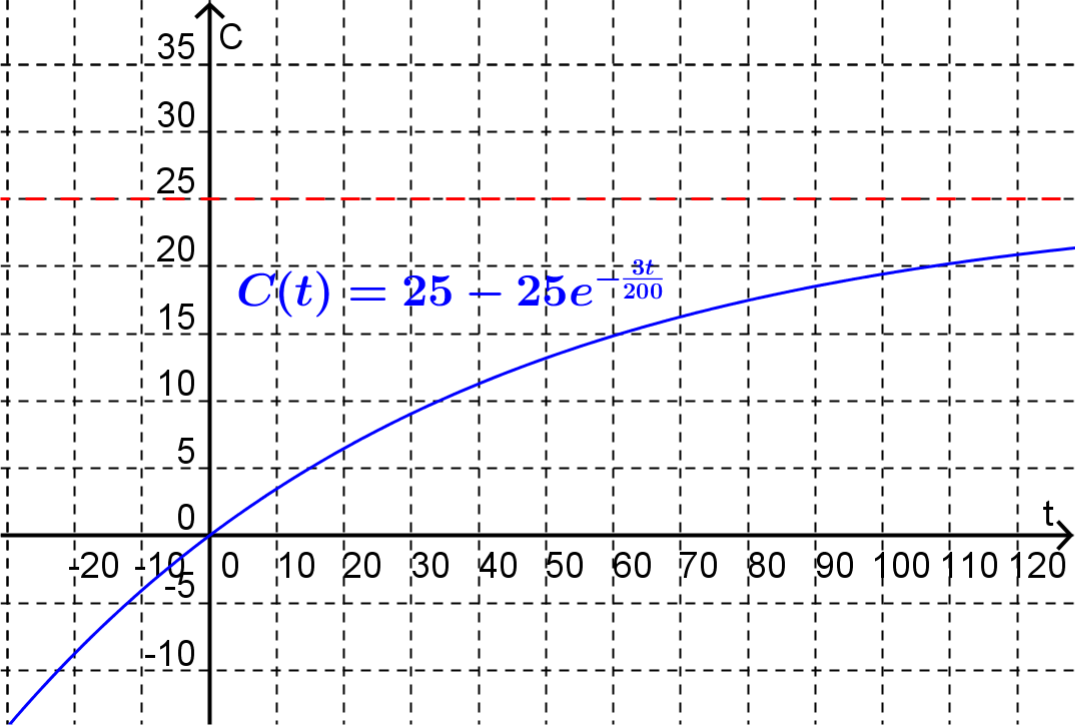
A \(200\)L tank contains pure water. At time \(t=0\) brackish water (i.e. water containing salt) begins to flow into the tank at a rate of \(3\)L/min and mixed water flows out at the same rate. Assuming that the concentration of salt in the inflowing water is \(25\)g/L determine the concentration of salt in the water in the tank as a function of time.
Answer.
\(C(t) = 25 - 25 \exp \left(- \dfrac{3}{200}t \right)\)
Solution.
Let \(C(t)\) be the concentration (in g/L) of the salt in the water in the tank at time \(t\) minutes after the mixing began and let \(A(t)\) be the amount (in grams) of salt in the tank at time \(t\text{.}\) Then \(C(0) = 0\) and \(A(0) = 0\text{.}\)
Now, salt is coming into the tank at the rate
\begin{equation*} 3 \times 25 = 75 \: \text{g/min}\text{,} \end{equation*}
and it is leaving the tank at the rate
\begin{equation*} 3 \times C(t) \: \text{g/min}\text{.} \end{equation*}
Thus \(A(t)\) will satisfy the DE
\begin{equation*} \dfrac{dA}{dt} = 75 - 3C\text{.} \end{equation*}
Using \(A(t) = 200 C(t)\) this becomes
\begin{equation*} 200 \dfrac{dC}{dt} = 75 - 3C \end{equation*}
which can be written as
\begin{equation*} \dfrac{dC}{dt} + \dfrac{3}{200}C = \dfrac{75}{200}\text{.} \end{equation*}
This is a first order linear DE and hence can be solved by multiplying the equation by the integrating factor
\begin{equation*} I(t) = \exp \left( \displaystyle \int \frac{3}{200} dt \right) = \exp \left( \dfrac{3}{200}t \right)\text{.} \end{equation*}
In doing this we obtain
\begin{equation*} \dfrac{d}{dt} \left[ \exp \left(\dfrac{3}{200} t \right) C \right] = \frac{75}{200} \exp \left( \dfrac{3}{200} t \right) \end{equation*}
and hence
\begin{equation*} \exp \left(\dfrac{3}{200}t \right) C = 25 \exp \left(\dfrac{3}{200}t \right) + K. \end{equation*}
Thus the general solution is
\begin{equation*} C(t) = 25 + K \exp\left( - \dfrac{3}{200} t \right)\text{.} \end{equation*}
Using \(C(0) = 0\) gives \(K = -25\) and so the required concentration function is
\begin{equation*} C(t) = 25 - 25 \exp \left(- \dfrac{3}{200}t \right)\text{.} \end{equation*}
Figure 11.13 shows a graph of this function. It can be seen that as \(t \to \infty\text{,}\) \(C \to 25\text{.}\) Thus as time goes by the concentration of salt in the tank water approaches the concentration of the salt in the brackish water coming into the tank.
Figure 11.13. Graph of \(C(t) = 25 - 25 \exp \left(- \dfrac{3}{200}t \right)\text{.}\)

Example 11.14. Motion in One Dimension.

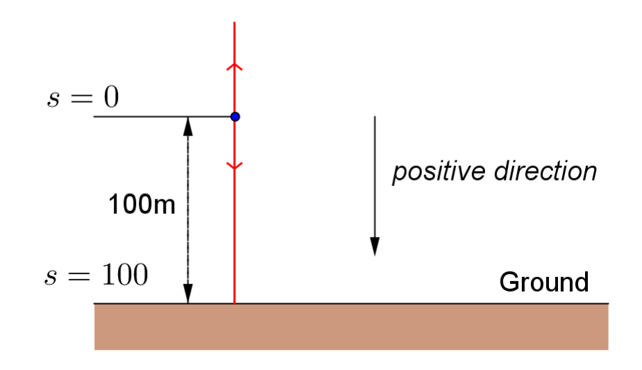
A ball of mass \(50\)kg is shot from a cannon \(100\)meters above the ground straight up with an initial velocity of \(10\)m/s. Assuming that the air resistance is given by \(5v\text{,}\) where \(v\) is the velocity, determine the velocity of the ball when it hits the ground.
Note: This is a very simple model for the air resistance chosen mostly to simplify the resultant equations
Answer.
\(v(5.98147) = 38.6 \, \text{m/s} \: (\text{to 1dp})\)
Solution.
Let \(v(t)\) be the velocity of the ball at time \(t\) seconds after it was fired from the cannon and let the downward direction be the positive direction as shown in Figure 11.15.
Figure 11.15.
The motion of the ball will be governed by Newton’s second law of motion which says
\begin{equation*} F = ma\text{,} \end{equation*}
where \(F\) is the net force acting on the ball, \(m\) is its mass and \(a\) is its acceleration. Once the ball leaves the cannon the forces acting on the ball are gravity, which we will denote by \(F_G\) and air resistance, denoted by \(F_R\text{.}\) Now with the positive direction as shown in Figure 11.15,
\begin{equation*} F_G = mg \end{equation*}
where \(g\) is the acceleration due to gravity. In the initial phase where the ball is going up the air resistance will be acting against the motion, (i.e. in the positive direction). Thus, since the velocity \(v\) is negative
\begin{equation*} F_R = -5v\text{.} \end{equation*}
In the second phase where the ball is falling the air resistance will again be acting against the motion (i.e. in the negative direction). In this phase the velocity is positive and so once again
\begin{equation*} F_R = -5v\text{.} \end{equation*}
Thus the net force acting on the ball is
\begin{equation*} F = F_G + F_R = mg-5v\text{.} \end{equation*}
Since
\begin{equation*} a = \dfrac{dv}{dt} \end{equation*}
Newton’s second law gives
\begin{equation*} m \dfrac{dv}{dt} = mg - 5v \end{equation*}
or
\begin{equation*} \dfrac{dv}{dt} + \dfrac{5}{m} v = g \end{equation*}
with
\begin{equation*} v(0) = -10\text{.} \end{equation*}
This is a first order linear DE in \(v(t)\text{.}\) To solve, multiply both sides of the DE by the integrating factor
\begin{equation*} I(t) = \exp \left( \displaystyle \int \frac{5}{m} dt \right) = \exp \left( \frac{5t}{m} \right) \end{equation*}
to get
\begin{equation*} \dfrac{d}{dt} \left[ \exp \left( \frac{5t}{m} v \right) \right] = g \exp \left( \frac{5t}{m} \right)\text{.} \end{equation*}
Integrating both sides gives
\begin{equation*} v(t) = \frac{mg}{5} + C \exp \left(-\frac{5t}{m} \right) \end{equation*}
and hence, using \(m=50\text{,}\) \(g=9.8\) and \(v(0) = -10\text{,}\)
\begin{equation*} v(t) = 98 - 108 e^{-t/10}\text{.} \end{equation*}
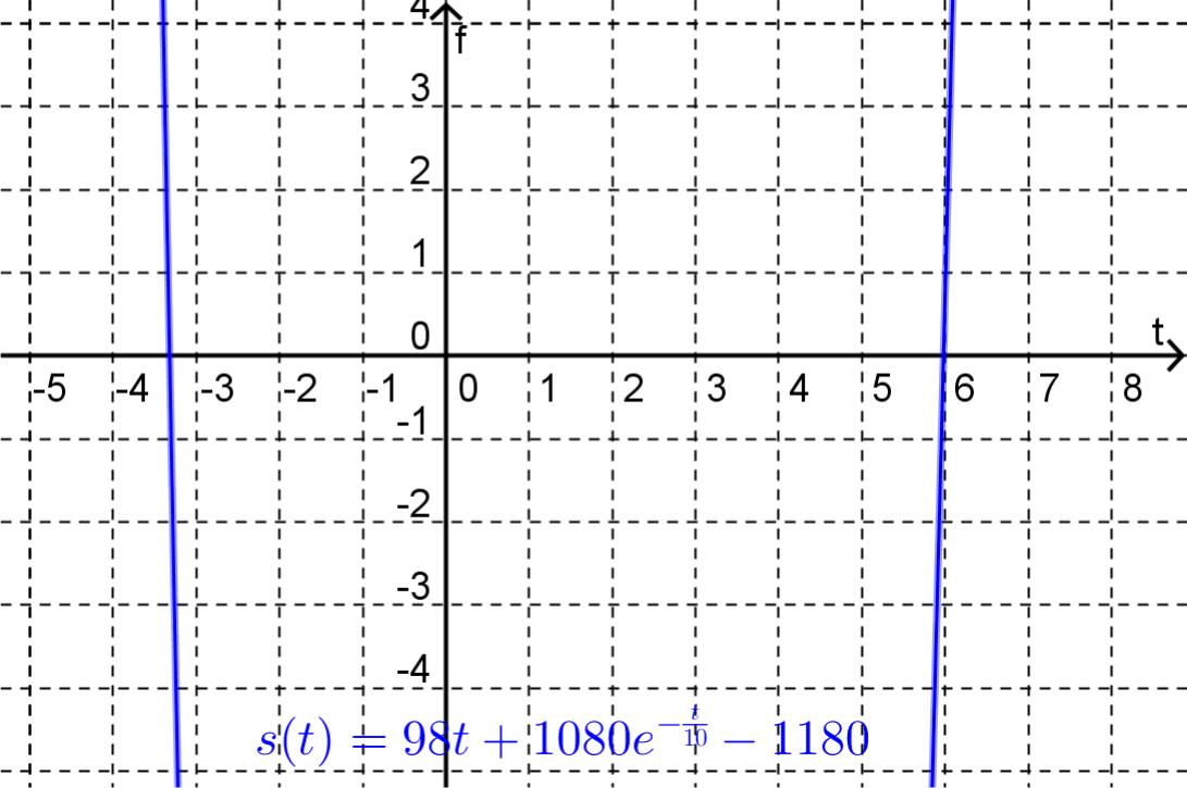
Thus we have determined the velocity function for the ball. To use this to determine the speed of the ball when it hits the ground we must first determine the time at which the ball hits the ground. To do this we will need the displacement function which we can obtain by integrating the velocity function. So, letting \(s(t)\) be the displacement of the ball at time \(t\text{,}\) we have
\begin{equation*} s(t) = \int v(t) \, dt = 98t + 1080e^{-t/10} + K \end{equation*}
Using \(s(0)=0\) gives \(K=-108\) and so the displacement function is
\begin{equation*} s(t) = 98t + 1080e^{-t/10} - 1080\text{.} \end{equation*}
Now \(s(t) = 100\) when
\begin{equation*} 98t + 1080e^{-t/10} - 1080 = 100\text{.} \end{equation*}
Figure 11.16 shows a plot of the function
\begin{equation*} f(t) = 98t + 1080e^{-t/10} - 1180 \end{equation*}
and as can be seen there is only one positive solution. Solving this equation numerically (using Newton’s method for example), shows this solution to be
\begin{equation*} t = 5.98147\text{.} \end{equation*}
Figure 11.16. Graph of \(s(t) = 98t + 1080e^{-t/10} -1180\text{.}\)
Thus the velocity of the ball when it hits the ground will be
\begin{equation*} v(5.98147) = 38.6 \, \text{m/s} \: (\text{to 1dp})\text{.} \end{equation*}

Exercises Example Tasks

1.
A population of insects in a region will grow at a rate that is proportional to their current population. In the absence of any outside factors the population will triple in two weeks time. On any given day there is a net migration into the area of \(15\) insects and \(16\) are eaten by the local bird population and \(7\) die of natural causes. If there are initially \(100\) insects in the area will the population survive? If not, when do they die out?
2.
A tank with a capacity of \(500\)L originally contains \(200\)L of water with \(10\)kg of salt in the solution. Water containing \(0.1\)kg of salt per litre is entering the tank at a rate of \(3\)L/min and the mixture is allowed to flow out of the tank at a rate of \(2\)L/min. Find the concentration of salt in the water in the tank at any time before the tank overflows.